This page was generated from a Jupyter notebook. You can download it here.

1D Action-Angle Coordinates and Inverse Transformations

galpy supports one-dimensional action-angle coordinates through actionAngleVertical and their inverse transformations through actionAngleVerticalInverse. These are useful for studying vertical oscillations in disk potentials or any general 1D potential.

For the special case of the harmonic oscillator, actionAngleHarmonic and actionAngleHarmonicInverse provide exact analytical action-angle coordinates and their inverse. These work like the other 1D classes described below, but only require the oscillator frequency \(\omega\).

from galpy.actionAngle import actionAngleHarmonic, actionAngleHarmonicInverse

aAH = actionAngleHarmonic(omega=1.0)
print("J =", aAH(1.0, 0.2))
print("(J, Omega) =", aAH.actionsFreqs(1.0, 0.2))
print("(J, Omega, angle) =", aAH.actionsFreqsAngles(1.0, 0.2))

J = 0.52
(J, Omega) = (0.52, np.float64(1.0))
(J, Omega, angle) = (0.52, np.float64(1.0), np.float64(1.373400766945016))

The inverse transformation recovers the original \((x, v_x)\):

aAHI = actionAngleHarmonicInverse(omega=1.0)
J, O, a = aAH.actionsFreqsAngles(1.0, 0.2)
print("(x, vx) =", aAHI(J, a))

(x, vx) = (np.float64(1.0), np.float64(0.19999999999999996))

For general (non-harmonic) 1D potentials, read on.

%matplotlib inline
import numpy
import matplotlib.pyplot as plt
import warnings

warnings.filterwarnings("ignore", category=RuntimeWarning)
warnings.filterwarnings("ignore", category=UserWarning)

actionAngleVertical

actionAngleVertical computes one-dimensional action-angle coordinates for vertical oscillations. We first need to extract a vertical potential from a 3D potential using toVerticalPotential.

from galpy.potential import toVerticalPotential, MWPotential2014

vp = toVerticalPotential(MWPotential2014, 1.0)

This extracts the vertical potential at \(R = 1\) (in natural units). Now we set up the actionAngleVertical object:

from galpy.actionAngle import actionAngleVertical

aAV = actionAngleVertical(pot=vp)

Computing actions, frequencies, and angles

The action-angle object can be called with (x, vx) to compute the action \(J\). The input is the vertical position and vertical velocity.

aAV(0.1, 0.1)

array([0.01231433])

To also get the frequency \(\Omega\), use actionsFreqs:

aAV.actionsFreqs(0.1, 0.1)

(array([0.01231433]), array([1.72942467]))

And to get the angle as well, use actionsFreqsAngles:

aAV.actionsFreqsAngles(0.1, 0.1)

(array([0.01231433]), array([1.72942467]), array([0.9955371]))

Action conservation along a 1D orbit

A key property of action variables is that they are conserved along an orbit. Let’s verify this by integrating a 1D orbit and computing the action at each time step.

from galpy.orbit import Orbit

o = Orbit([0.1, 0.1])  # 1D orbit: (x, vx)
ts = numpy.linspace(0.0, 20.0, 1001)
o.integrate(ts, vp)

Now compute the action at each time step and verify conservation:

# Compute the action at each time step
actions = aAV(o.x(ts), o.vx(ts))
plt.plot(ts, actions)
plt.xlabel(r"$t$")
plt.ylabel(r"$J$")
plt.title("Action conservation along a 1D orbit")
plt.ylim(actions.mean() - 0.01, actions.mean() + 0.01);

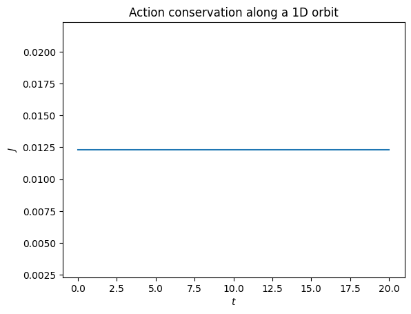
The action is conserved to high precision along the orbit, as expected.

actionAngleVerticalInverse

actionAngleVerticalInverse computes the reverse transformation: from action-angle coordinates \((J, \theta)\) back to phase-space coordinates \((x, v_x)\). This is useful for constructing tori in 1D potentials.

We demonstrate this with the IsothermalDiskPotential.

from galpy.potential import IsothermalDiskPotential

ip = IsothermalDiskPotential(amp=1.0, sigma=0.6)

Set up the inverse action-angle object. The nta parameter controls the number of angle points used internally, and Es specifies the energies for which to set up the transformation. Using setup_interp=True enables interpolation between tori at different energies.

from galpy.actionAngle import actionAngleVerticalInverse

aAVI = actionAngleVerticalInverse(
    pot=ip,
    nta=512,
    Es=numpy.linspace(0.05, 1.0, 10),
    setup_interp=True,
)

Evaluating the inverse transformation

We can evaluate the transformation to get \((x, v_x)\) from a given action \(J\) and an array of angles \(\theta\).

angles = numpy.linspace(0, 2 * numpy.pi, 100)
x, vx = aAVI(0.1, angles)

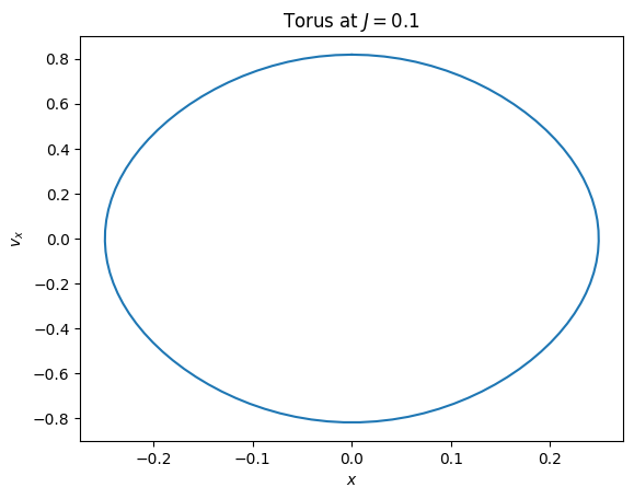
Plotting the torus

The resulting \((x, v_x)\) pairs trace out a torus (a closed curve in 1D phase space).

plt.plot(x, vx)
plt.xlabel(r"$x$")
plt.ylabel(r"$v_x$")
plt.title(r"Torus at $J = 0.1$");

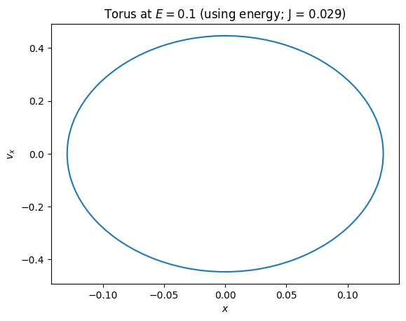
You can also specify a torus using its energy instead by using the aA1Dinv.J method:

x, vx = aAVI(aAVI.J(0.1), angles)
plt.plot(x, vx)
plt.xlabel(r"$x$")
plt.ylabel(r"$v_x$")
plt.title(rf"Torus at $E = 0.1$ (using energy; J = {aAVI.J(0.1):.3f})");

We can also plot tori at multiple action values to visualize the phase-space structure:

angles = numpy.linspace(0, 2 * numpy.pi, 200)
for J in [0.05, 0.1, 0.2, 0.3]:
    x, vx = aAVI(J, angles)
    plt.plot(x, vx, label=rf"$J = {J}$")
plt.xlabel(r"$x$")
plt.ylabel(r"$v_x$")
plt.legend()
plt.title("Tori at different action values");

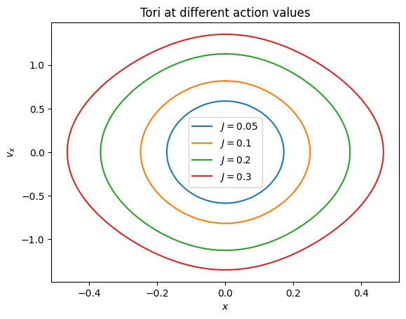
The setup_interp=True option allows smooth interpolation between the tori computed at the specified energies, enabling evaluation at arbitrary action values within the range covered by those energies.