This page was generated from a Jupyter notebook. You can download it here.

Two-dimensional Disk Distribution Functions

galpy includes several distribution functions (DFs) for razor-thin axisymmetric disks: dehnendf (Dehnen 1999), shudf (Shu 1969), and schwarzschilddf (the Shu DF in the epicycle approximation, see galaxiesbook.org). These DFs are functions of energy and angular momentum, \(f(E, L_z)\), and can be used to describe stellar populations in a thin disk with a flat or power-law rotation curve.

%matplotlib inline
import numpy
import matplotlib.pyplot as plt
from galpy.util.quadpack import AccuracyWarning
import warnings

warnings.filterwarnings("ignore", category=RuntimeWarning)
warnings.filterwarnings("ignore", category=UserWarning)
warnings.filterwarnings("ignore", category=AccuracyWarning)

Types of 2D disk DFs

All three DFs assume an exponential surface-density profile and an exponential velocity-dispersion profile by default. They differ in how they construct \(f(E, L_z)\) (see Section 10.2.2 in galaxiesbook.org for more details):

• dehnendf: Dehnen’s ‘new’ DF (Dehnen 1999)

• shudf: Shu’s DF (Shu 1969)

• schwarzschilddf: Schwarzschild DF

All operate in a potential with a power-law rotation curve \(v_c \propto R^\beta\).

Initializing a Dehnen DF

We initialize a dehnendf with a flat rotation curve (beta=0.). The default profileParams=(1/3, 1, 0.2) set the disk scale length, velocity-dispersion scale length, and velocity dispersion at \(R_0\) (all in natural units).

from galpy.df import dehnendf

dfc = dehnendf(beta=0.0)

The profileParams tuple is (xD, xS, Sro) where:

• xD = 1/3: disk surface mass scale length (in units of \(R_0\))

• xS = 1.0: velocity dispersion scale length

• Sro = 0.2: velocity dispersion at \(R_0\) (in units of \(v_c(R_0)\))

We can also use custom profile parameters:

dfc2 = dehnendf(beta=0.0, profileParams=(1.0 / 3.0, 1.0, 0.15))

Evaluating the DF for an orbit

The DF can be evaluated for a given orbit (a point in phase space). We create an Orbit object and pass it to the DF:

from galpy.orbit import Orbit

# An orbit at R=0.9, vR=0.05, vT=1.0
o = Orbit([0.9, 0.05, 1.0])
print("f(orbit) =", dfc(o))

f(orbit) = 0.3014411904461411

DF moments: surface mass, velocity dispersions, and mean velocities

We can compute various moments of the DF by marginalizing over velocity. These are useful for comparing the DF to observations.

# Surface mass density at R=1
print("Surface mass at R=1.0:", dfc.surfacemass(1.0))

# Radial velocity dispersion squared
print("sigma_R^2 at R=1.0:", dfc.sigma2(1.0))

# Mean tangential velocity
print("<v_T> at R=1.0:", dfc.meanvT(1.0))

# Mean radial velocity (should be ~0 for an axisymmetric DF)
print("<v_R> at R=1.0:", dfc.meanvR(1.0))

Surface mass at R=1.0: 0.050968080499022066
sigma_R^2 at R=1.0: 0.03733043742309621
<v_T> at R=1.0: 0.9171527697944728
<v_R> at R=1.0: 0.0

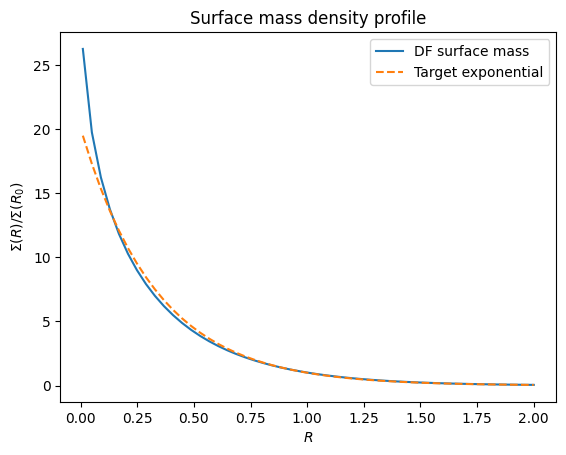
Let’s plot the surface mass profile and compare it to the target exponential profile:

Rs = numpy.linspace(0.01, 2.0, 51)
smass = numpy.array([dfc.surfacemass(R) for R in Rs])
plt.plot(Rs, smass / smass[25], label="DF surface mass")
plt.plot(Rs, numpy.exp(-(Rs - 1.0) / (1.0 / 3.0)), "--", label="Target exponential")
plt.xlabel(r"$R$")
plt.ylabel(r"$\Sigma(R) / \Sigma(R_0)$")
plt.legend()
plt.title("Surface mass density profile");

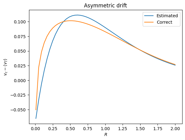
Asymmetric drift

The asymmetric drift is the difference between the circular velocity and the mean tangential velocity: \(v_c - \langle v_T \rangle\). The DF can calculate this directly as \(v_c - \langle v_T \rangle\) or we can also estimate this from an approximation to the Jeans equation using asymmetricdrift (see galaxiesbook.org for more details):

print(f"Estimated asymmetric drift at R=1.0: {dfc.asymmetricdrift(1.0)}")
print(f" vs. correct one from mean tangential velocity: {1.0 - dfc.meanvT(1.0)}")

# Plot asymmetric drift as a function of R
ad = numpy.array([dfc.asymmetricdrift(R) for R in Rs])
ad_correct = numpy.array([1.0 - dfc.meanvT(R) for R in Rs])
plt.plot(Rs, ad, label="Estimated")
plt.plot(Rs, ad_correct, label="Correct")
plt.xlabel(r"$R$")
plt.ylabel(r"$v_c - \langle v_T \rangle$")
plt.title("Asymmetric drift")
plt.legend();

Estimated asymmetric drift at R=1.0: 0.09000000000000002
 vs. correct one from mean tangential velocity: 0.0828472302055272

Sampling orbits from the DF

We can draw random samples from the DF. The sample method returns Orbit objects:

numpy.random.seed(1)
samples = dfc.sample(n=500, returnOrbit=True, nphi=1)
print("Number of sampled orbits:", len(samples))
print("First orbit R, vR, vT:", samples[0].R(), samples[0].vR(), samples[0].vT())

Number of sampled orbits: 500
First orbit R, vR, vT: 0.24207749508260903 0.5832560359657737 0.633604070684058

Plotting the velocity distribution

We can sample velocities at a specific radius and plot their distribution. The sampleVRVT method samples \((v_R, v_T)\) at a given \(R\):

numpy.random.seed(1)
vrvt = dfc.sampleVRVT(1.0, n=1000)
plt.scatter(vrvt[:, 0], vrvt[:, 1], s=1, alpha=0.5, label="Samples")

# Evaluate DF on a (vR, vT) grid at R=1 and overplot contours
vR_grid = numpy.linspace(vrvt[:, 0].min() - 0.1, vrvt[:, 0].max() + 0.1, 60)
vT_grid = numpy.linspace(vrvt[:, 1].min() - 0.1, vrvt[:, 1].max() + 0.1, 60)
vR2d, vT2d = numpy.meshgrid(vR_grid, vT_grid)

df_grid = numpy.array([[dfc(Orbit([1.0, vR, vT])) for vR in vR_grid] for vT in vT_grid])

levels = numpy.geomspace(0.02 * df_grid.max(), 0.9 * df_grid.max(), 6)
plt.contour(vR2d, vT2d, df_grid, levels=levels, colors="k", linewidths=1.0)

plt.xlabel(r"$v_R$")
plt.ylabel(r"$v_T$")
plt.title("Velocity distribution at R=1")
plt.axhline(1.0, color="r", ls="--", label=r"$v_c$")
plt.legend();

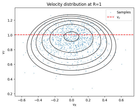
The distribution is centered slightly below \(v_c = 1\) due to the asymmetric drift, and has a spread set by the velocity dispersion.

Other 2D DFs

The shudf and schwarzschilddf classes have the same interface:

from galpy.df import shudf, schwarzschilddf

dfs = shudf(beta=0.0)
dfsw = schwarzschilddf(beta=0.0)

print("Shu DF surface mass at R=1:", dfs.surfacemass(1.0))
print("Schwarzschild DF surface mass at R=1:", dfsw.surfacemass(1.0))

Shu DF surface mass at R=1: 0.062193623796354555
Schwarzschild DF surface mass at R=1: 0.0689371283692479

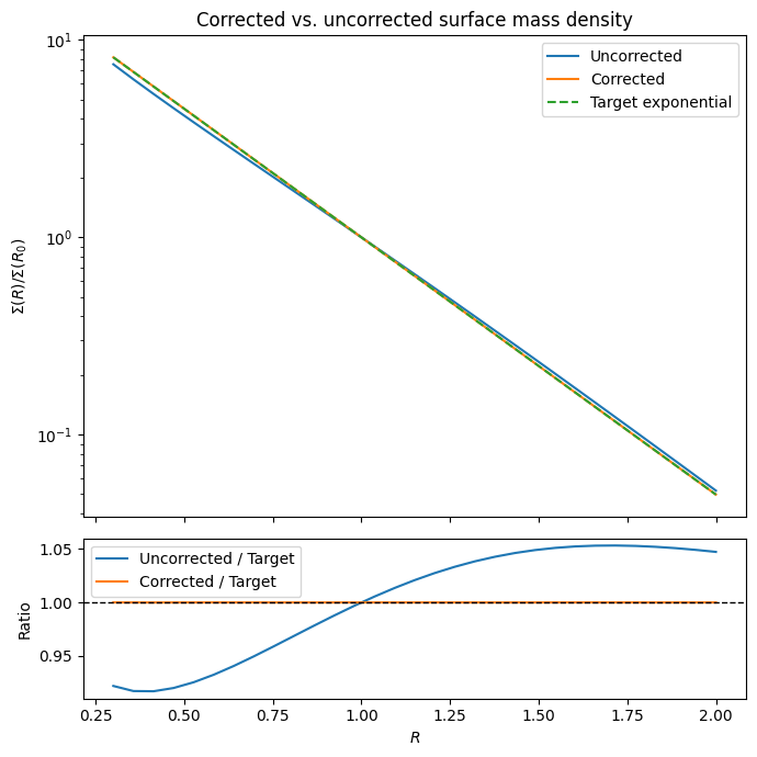
Corrected DFs

The input profiles are only approximately reproduced by the DF. We can correct this by calculating a set of corrections (see Dehnen 1999). galpy supports these corrections and comes with pre-calculated corrections bundled with the code:

dfc_corr = dehnendf(beta=0.0, correct=True)

# The corrected DF reproduces the target velocity dispersion much better
print(
    "sigma_R (corrected vs. uncorrected):",
    numpy.sqrt(dfc_corr.sigmaR2(1.0)),
    numpy.sqrt(dfc.sigmaR2(1.0)),
)
print("meanvT (corrected vs. uncorrected):", dfc_corr.meanvT(1.0), dfc.meanvT(1.0))

# Compare surface mass profiles and ratios to target
Rs = numpy.linspace(0.3, 2.0, 31)
smass_uncorr = numpy.array([dfc.surfacemass(R) for R in Rs]) / dfc.surfacemass(1.0)
smass_corr = numpy.array([dfc_corr.surfacemass(R) for R in Rs]) / dfc_corr.surfacemass(
    1.0
)
target = numpy.exp(-(Rs - 1.0) / (1.0 / 3.0))

fig, (ax1, ax2) = plt.subplots(
    2, 1, sharex=True, figsize=(7, 7), gridspec_kw={"height_ratios": [3, 1]}
)

# Top panel: profiles
ax1.semilogy(Rs, smass_uncorr, label="Uncorrected")
ax1.semilogy(Rs, smass_corr, label="Corrected")
ax1.semilogy(Rs, target, "--", label="Target exponential")
ax1.set_ylabel(r"$\Sigma(R) / \Sigma(R_0)$")
ax1.set_title("Corrected vs. uncorrected surface mass density")
ax1.legend()

# Bottom panel: ratio to target
ax2.plot(Rs, smass_uncorr / target, label="Uncorrected / Target")
ax2.plot(Rs, smass_corr / target, label="Corrected / Target")
ax2.axhline(1.0, color="k", ls="--", lw=1)
ax2.set_xlabel(r"$R$")
ax2.set_ylabel("Ratio")
ax2.legend()

plt.tight_layout()

sigma_R (corrected vs. uncorrected): 0.1999998506941359 0.19321086259083936
meanvT (corrected vs. uncorrected): 0.9035516117477274 0.9171527697944728

galpy will automatically save any new corrections that you calculate.

Oort constants

galpy can calculate the Oort constants (A, B, C, K) for 2D disk DFs by direct integration over the DF and its derivatives:

print("Oort A:", dfc.oortA(1.0))
print("Oort B:", dfc.oortB(1.0))
print("Oort C:", dfc.oortC(1.0))  # zero for axisymmetric DFs
print("Oort K:", dfc.oortK(1.0))  # zero for axisymmetric DFs
# In the epicycle approximation for a flat rotation curve, A = -B = 0.5
print(
    "A + B (should be ~0 for cold DF w/ flat rotation curve):",
    dfc.oortA(1.0) + dfc.oortB(1.0),
)

# For a cold DF, the epicycle approximation is better:
dfccold = dehnendf(beta=0.0, profileParams=(1.0 / 3.0, 1.0, 0.02))
print("Cold DF: A =", dfccold.oortA(1.0), ", B =", dfccold.oortB(1.0))

Oort A: 0.4319078088921877
Oort B: -0.4852449609022851
Oort C: 0.0
Oort K: 0.0
A + B (should be ~0 for cold DF w/ flat rotation curve): -0.053337152010097366
Cold DF: A = 0.4991755666614268 , B = -0.4999282474249216

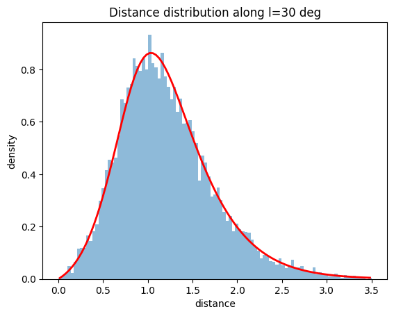
Line-of-sight sampling

galpy supports sampling along a given line of sight in the disk, useful for interpreting surveys with a finite number of pointings:

# Sample distances along a line of sight at l=30 degrees
ds = dfc.sampledSurfacemassLOS(30.0 / 180.0 * numpy.pi, n=10000)
hists, bins, edges = plt.hist(ds, range=[0.0, 3.5], density=True, bins=101, alpha=0.5)
# Compare to the predicted distribution
xs = numpy.array([(bins[ii + 1] + bins[ii]) / 2.0 for ii in range(len(bins) - 1)])
fd = numpy.array([dfc.surfacemassLOS(d, 30.0) for d in xs])
plt.plot(xs, fd / numpy.sum(fd) / (xs[1] - xs[0]), "r-", lw=2)
plt.xlabel("distance")
plt.ylabel("density")
plt.title("Distance distribution along l=30 deg");

Non-axisymmetric, time-dependent DFs: evolveddiskdf

galpy supports evaluation of non-axisymmetric, time-dependent 2D DFs. These are constructed by assuming an initial axisymmetric steady state that is then acted upon by a non-axisymmetric perturbation. The DF at any time is evaluated by integrating orbits backwards to the initial time (using Liouville’s theorem). This is implemented as galpy.df.evolveddiskdf.

from galpy.potential import LogarithmicHaloPotential, EllipticalDiskPotential
from galpy.df import evolveddiskdf

# Set up an elliptical perturbation to a logarithmic potential
lp = LogarithmicHaloPotential(normalize=1.0)
ep = EllipticalDiskPotential(twophio=0.05, phib=0.0, p=0.0, tform=-150.0, tsteady=125.0)

# Initial steady-state DF (warm disk)
idfwarm = dehnendf(beta=0.0, profileParams=(1.0 / 3.0, 1.0, 0.15))

# Set up the evolved DF
edfwarm = evolveddiskdf(idfwarm, lp + ep, to=-150.0)

# Mean radial velocity at R=0.9, phi=22.5 deg
mvrwarm, gridwarm = edfwarm.meanvR(
    0.9, phi=22.5, deg=True, t=0.0, grid=True, returnGrid=True, gridpoints=51
)
print("Mean v_R (warm disk):", mvrwarm)

Mean v_R (warm disk): -0.029476364282585484

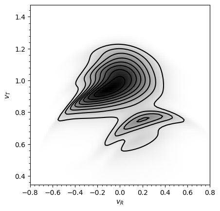
Example: The Hercules stream

We can combine galpy’s orbit integration capabilities with the disk distribution functions to see the effect of the Galactic bar on stellar velocities. By backward-integrating orbits starting at the Solar position in a potential that includes the bar, we can see what the velocity distribution should look like today if the Galactic bar stirred up a steady-state disk (see Dehnen 2000 and Bovy 2010).

from galpy.potential import LogarithmicHaloPotential, DehnenBarPotential
from galpy.df import dehnendf

lp = LogarithmicHaloPotential(normalize=1.0)
dp = DehnenBarPotential()

# Integrate back to before bar formation
ts = numpy.linspace(0, dp.tform(), 1000)

# Grid in velocity space at the Solar position
ins = Orbit(
    numpy.array(
        [
            [
                [1.0, -0.7 + 1.4 / 100 * jj, 1.0 - 0.6 + 1.2 / 100 * ii, 0.0]
                for jj in range(101)
            ]
            for ii in range(101)
        ]
    )
)
ins.integrate(ts, lp + dp)

Evaluate the weight of each orbit using a Dehnen DF at the time of bar formation:

dfc = dehnendf(beta=0.0, correct=True)
out = [[dfc(o(dp.tform())) for o in j] for j in ins]
out = numpy.array(out)

Plot the velocity distribution:

from galpy.util.plot import dens2d

dens2d(
    out,
    origin="lower",
    cmap="gist_yarg",
    contours=True,
    xrange=[-0.7, 0.7],
    yrange=[0.4, 1.6],
    xlabel=r"$v_R$",
    ylabel=r"$v_T$",
);

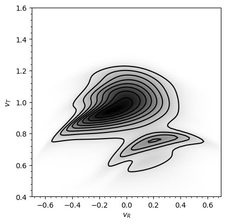
This entire calculation is encapsulated in the evolveddiskdf module:

from galpy.df import evolveddiskdf

edf = evolveddiskdf(dfc, lp + dp, to=dp.tform())
mvr, grid = edf.meanvR(1.0, grid=True, gridpoints=101, returnGrid=True)
dens2d(
    grid.df.T,
    origin="lower",
    cmap="gist_yarg",
    contours=True,
    xrange=[grid.vRgrid[0], grid.vRgrid[-1]],
    yrange=[grid.vTgrid[0], grid.vTgrid[-1]],
    xlabel=r"$v_R$",
    ylabel=r"$v_T$",
);

The Hercules stream is the feature at \((v_R, v_T) \approx (-0.3, 0.8)\). Note that the \(v_R\) axis here is defined as the negative of the convention in Dehnen (2000) and Bovy (2010).