This page was generated from a Jupyter notebook. You can download it here.
Spherical Distribution Functions
galpy includes several distribution functions for spherical systems, both isotropic and anisotropic. These DFs are tied to a specific spherical potential and can be used to compute properties of the system or to generate samples. galpy contains a number of specific isotropic and anisotropic DFs, but it also includes a general classes for computing the DF of any spherical system using Eddington’s formula for isotropic systems and similar formulas for anisotropic systems with constant anisotropy or anisotropy of the Osipkov-Merritt type. See galaxiesbook.org for more details on these DFs and the underlying theory.
[1]:
%matplotlib inline
import numpy
import matplotlib.pyplot as plt
from galpy.util.quadpack import AccuracyWarning
import warnings

warnings.filterwarnings("ignore", category=RuntimeWarning)
warnings.filterwarnings("ignore", category=UserWarning)
warnings.filterwarnings("ignore", category=AccuracyWarning)
Isotropic Hernquist DF
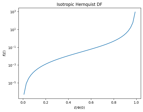
The isotropicHernquistdf is initialized from a HernquistPotential instance. The DF is a function of energy only, \(f(E)\), corresponding to an isotropic velocity distribution.
[2]:
from galpy.potential import HernquistPotential
from galpy.df import isotropicHernquistdf

hp = HernquistPotential(amp=2.0, a=1.3)
dfh = isotropicHernquistdf(pot=hp)
Evaluating the DF as a function of energy
The DF can be evaluated at a given (relative) energy \(E\). The relative energy is defined as \(E = \Psi(r) - \frac{1}{2}v^2\) where \(\Psi = -\Phi\) is the relative potential:
[3]:
# Evaluate at several energies
Es = numpy.linspace(0.01, 0.99, 50)
# Scale by Phi(0) to get the DF as a function of energy
phi0 = hp(0.0, 0.0, use_physical=False)
fE = numpy.array([dfh.fE(E * phi0) for E in Es])
plt.semilogy(Es, fE)
plt.xlabel(r"$E / \Phi(0)$")
plt.ylabel(r"$f(E)$")
plt.title("Isotropic Hernquist DF");
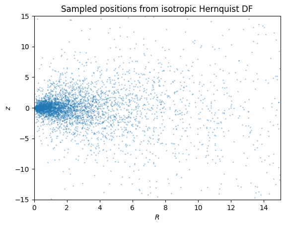
Sampling positions and velocities
The sample method draws random phase-space points from the DF. By default it returns an Orbit object:
[4]:
numpy.random.seed(1)
samples = dfh.sample(n=5000)
print("Type:", type(samples))
print("Number of orbits:", len(samples))
Type: <class 'galpy.orbit.Orbits.Orbit'>
Number of orbits: 5000
Let’s plot the spatial distribution of the sampled orbits:
[5]:
# Plot the spatial distribution
Rs = samples.R()
zs = samples.z()
plt.scatter(Rs, zs, s=1, alpha=0.3)
plt.xlabel(r"$R$")
plt.ylabel(r"$z$")
plt.title("Sampled positions from isotropic Hernquist DF")
plt.xlim(0, 15)
plt.ylim(-15, 15);
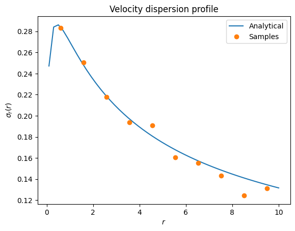
Velocity dispersion profile
We can compare the velocity dispersion profile of the samples to the analytical prediction. The sigmar method computes \(\sigma_r(r)\):
[6]:
# Analytical velocity dispersion
rs = numpy.linspace(0.1, 10.0, 50)
sigmar = numpy.array([dfh.sigmar(r) for r in rs])

# Velocity dispersion from samples
r_samples = samples.r()
vr_samples = (
    samples.x() * samples.vx() + samples.y() * samples.vy() + samples.z() * samples.vz()
) / r_samples

# Bin the samples
rbins = numpy.linspace(0.1, 10.0, 11)
rmid = 0.5 * (rbins[:-1] + rbins[1:])
sig_binned = numpy.zeros(len(rmid))
for i in range(len(rmid)):
    mask = (r_samples >= rbins[i]) & (r_samples < rbins[i + 1])
    if numpy.sum(mask) > 2:
        sig_binned[i] = numpy.std(vr_samples[mask])

plt.plot(rs, sigmar, label="Analytical")
plt.plot(rmid, sig_binned, "o", label="Samples")
plt.xlabel(r"$r$")
plt.ylabel(r"$\sigma_r(r)$")
plt.legend()
plt.title("Velocity dispersion profile");
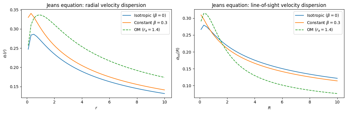
Jeans equation tools
galpy also provides tools for computing velocity moments from the Jeans equation in galpy.df.jeans. These are useful for comparing with DF-based calculations and for quick estimates when a full DF is not needed.
The main functions are:
jeans.sigmar(pot, r): radial velocity dispersion \(\sigma_r(r)\)jeans.sigmalos(pot, R): line-of-sight velocity dispersion \(\sigma_\mathrm{los}(R)\)
Both of these functions allow the user to specify the anisotropy profile \(\beta(r)\), which is defined as \(\beta(r) = 1 - \frac{\sigma_\theta^2 + \sigma_\phi^2}{2\sigma_r^2}\) as well as the tracer density profile \(\nu(r)\), which is needed to solve the Jeans equation. By default, beta is set to 0 (isotropic) and nu is set to the density profile of the potential.
[7]:
from galpy.df import jeans

# Compute radial velocity dispersion from the Jeans equation
rs_jeans = numpy.linspace(0.1, 10.0, 50)
sigmar_jeans = numpy.array([jeans.sigmar(hp, r, use_physical=False) for r in rs_jeans])

# Compute for constant beta=0.3
sigmar_jeans_b03 = numpy.array(
    [jeans.sigmar(hp, r, beta=0.3, use_physical=False) for r in rs_jeans]
)

# Compute for Osipkov-Merritt-style beta(r) = r^2/(r^2 + ra^2)
beta_om = lambda r: r**2 / (r**2 + 1.4**2)
sigmar_jeans_om = numpy.array(
    [jeans.sigmar(hp, r, beta=beta_om, use_physical=False) for r in rs_jeans]
)

# Compute line-of-sight velocity dispersion
sigmalos_jeans = numpy.array(
    [jeans.sigmalos(hp, R, use_physical=False) for R in rs_jeans]
)
sigmalos_jeans_b03 = numpy.array(
    [jeans.sigmalos(hp, R, beta=0.3, use_physical=False) for R in rs_jeans]
)
sigmalos_jeans_om = numpy.array(
    [jeans.sigmalos(hp, R, beta=beta_om, use_physical=False) for R in rs_jeans]
)

fig, axes = plt.subplots(1, 2, figsize=(12, 4))
axes[0].plot(rs_jeans, sigmar_jeans, label=r"Isotropic ($\beta=0$)")
axes[0].plot(rs_jeans, sigmar_jeans_b03, label=r"Constant $\beta=0.3$")
axes[0].plot(rs_jeans, sigmar_jeans_om, "--", label=r"OM ($r_a=1.4$)")
axes[0].set_xlabel(r"$r$")
axes[0].set_ylabel(r"$\sigma_r(r)$")
axes[0].set_title("Jeans equation: radial velocity dispersion")
axes[0].legend()

axes[1].plot(rs_jeans, sigmalos_jeans, label=r"Isotropic ($\beta=0$)")
axes[1].plot(rs_jeans, sigmalos_jeans_b03, label=r"Constant $\beta=0.3$")
axes[1].plot(rs_jeans, sigmalos_jeans_om, "--", label=r"OM ($r_a=1.4$)")
axes[1].set_xlabel(r"$R$")
axes[1].set_ylabel(r"$\sigma_\mathrm{los}(R)$")
axes[1].set_title("Jeans equation: line-of-sight velocity dispersion")
axes[1].legend()
fig.tight_layout();
King DF
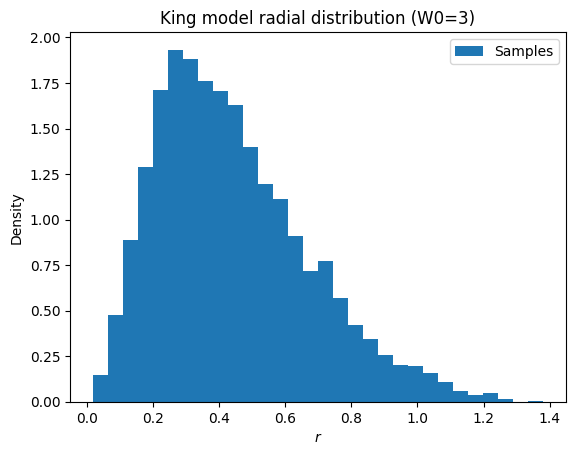
The King DF models a tidally-truncated, lowered-isothermal distribution. It is initialized with the dimensionless central potential \(W_0\), total mass, and tidal radius:
[8]:
numpy.random.seed(1)
from galpy.df import kingdf

kdf = kingdf(W0=3.0, M=1.0, rt=1.5)

# Sample from the King model
king_samples = kdf.sample(n=5000)
r_king = king_samples.r()
plt.hist(r_king, bins=30, density=True, label="Samples")
plt.xlabel(r"$r$")
plt.ylabel("Density")
plt.title("King model radial distribution (W0=3)")
plt.legend();
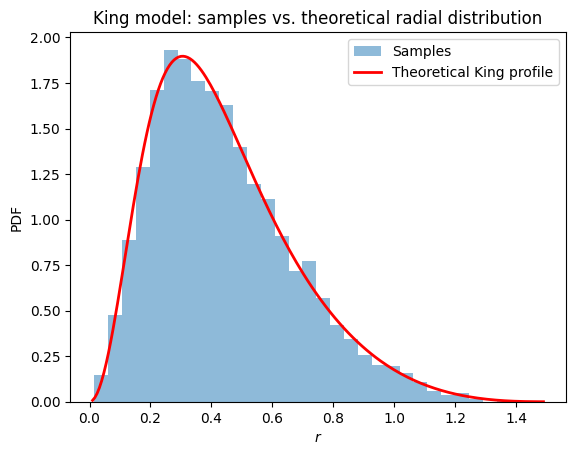
We can compare the sampled radial distribution with the theoretical King density profile. The King DF provides a dens(r) method that returns the density at a given radius. To compare with the histogram of radii, we need to weight by the volume element \(4\pi r^2\):
[9]:
# Theoretical King density profile weighted by volume element
r_theory = numpy.linspace(0.01, 1.49, 200)
rho_theory = numpy.array([kdf.dens(r) for r in r_theory])
# The histogram shows the PDF of radii, which is proportional to rho(r) * 4*pi*r^2
radial_pdf = rho_theory * 4.0 * numpy.pi * r_theory**2
# Normalize to integrate to 1 (since histogram is density=True)
from scipy import integrate

radial_pdf /= integrate.trapezoid(radial_pdf, r_theory)

plt.hist(r_king, bins=30, density=True, alpha=0.5, label="Samples")
plt.plot(r_theory, radial_pdf, "r-", lw=2, label="Theoretical King profile")
plt.xlabel(r"$r$")
plt.ylabel("PDF")
plt.title("King model: samples vs. theoretical radial distribution")
plt.legend();
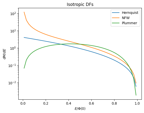
Differential energy distribution
galpy can also compute the differential energy distribution \(N(E)\), which is the number of stars per unit energy. This is related to the DF by integrating over phase space at fixed energy:
[10]:
hp = HernquistPotential(amp=2.0, a=1.3)
dfh = isotropicHernquistdf(pot=hp)

from galpy.potential import NFWPotential, PlummerPotential
from galpy.df import isotropicNFWdf, isotropicPlummerdf

nfp = NFWPotential(amp=1.0, a=1.0)
dfnfw = isotropicNFWdf(pot=nfp)
pp = PlummerPotential(amp=1.0, b=1.0)
dfplummer = isotropicPlummerdf(pot=pp)

# Evaluate at several energies
Es = numpy.linspace(0.01, 0.99, 50)
# Scale by Phi(0) to get the DF as a function of energy
phi0_hp = hp(0.0, 0.0, use_physical=False)
dMdE_hp = numpy.array([dfh.dMdE(E * phi0_hp) for E in Es])
phi0_nfw = nfp(0.0, 0.0, use_physical=False)
dMdE_nfw = numpy.array([dfnfw.dMdE(E * phi0_nfw) for E in Es])
phi0_plummer = pp(0.0, 0.0, use_physical=False)
dMdE_plummer = numpy.array([dfplummer.dMdE(E * phi0_plummer) for E in Es])
plt.semilogy(Es, dMdE_hp, label="Hernquist")
plt.semilogy(Es, dMdE_nfw, label="NFW")
plt.semilogy(Es, dMdE_plummer, label="Plummer")
plt.xlabel(r"$E / \Phi(0)$")
plt.ylabel(r"$dM/dE$")
plt.title("Isotropic DFs")
plt.legend();
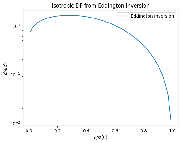
Using the Eddington inversion
The eddingtondf class can be used to compute the isotropic DF for any spherical potential using Eddington’s formula. This is useful for potentials that do not have an analytical DF, for comparing with the analytical DFs of specific potentials, or for computing the DFs of tracers in a given potential, e.g., a Hernquist population in an NFW potential. We give an example of the latter here:
[11]:
from galpy.df import eddingtondf

nfp = NFWPotential(amp=1.0, a=1.0)
hp = HernquistPotential(amp=2.0, a=1.3)
df_edd = eddingtondf(pot=nfp, denspot=hp)
Es = numpy.linspace(0.01, 0.99, 50)
phi0_nfw = nfp(0.0, 0.0, use_physical=False)
dMdE_edd = numpy.array([df_edd.dMdE(E * phi0_nfw) for E in Es])
plt.semilogy(Es, dMdE_edd, label="Eddington inversion")
plt.xlabel(r"$E / \Phi(0)$")
plt.ylabel(r"$dM/dE$")
plt.title("Isotropic DF from Eddington inversion")
plt.legend();
N-body initial conditions for a truncated NFW halo
A common application of these sampling tools is setting up N-body initial conditions for a dark-matter halo in equilibrium. The NFW profile is the standard choice, but it has a well-known problem for this purpose: its enclosed mass grows like \(M(<r) \propto \ln(1+r/a) - (r/a)/(1+r/a)\), which diverges logarithmically as \(r \to \infty\). The total mass is therefore infinite and there is no normalizable density from which to draw a finite set of particles, so the profile must be truncated somewhere.
galpy provides the ExpTruncNFWPotential, which multiplies the NFW density by an exponential cutoff \(e^{-r/r_c}\). This gives a finite total mass while leaving the inner cusp unchanged. The convenient from_nfw constructor truncates an existing NFWPotential; here we set the truncation (cutoff) radius to the virial radius (\(r_c = r_\mathrm{vir}\)), the natural boundary of a halo. Because the exponential cutoff is gradual rather than
a hard edge, an appreciable fraction of the mass lies beyond \(r_\mathrm{vir}\), so when sampling we extend the distribution function out to a few times the cutoff radius (\(r_\mathrm{max} = 3\,r_\mathrm{vir}\) below). This captures \(\approx 99\%\) of the total mass, whereas cutting the DF off at \(r_\mathrm{vir}\) itself would discard \(\sim 15\%\) of it.
[12]:
from galpy.potential import NFWPotential, ExpTruncNFWPotential
from galpy.df import eddingtondf
from astropy import units as u

# A Milky-Way-mass NFW halo (M_vir = 1e12 Msun, concentration 10)
nfw = NFWPotential(mvir=1.0, conc=10.0, ro=8.0, vo=220.0)
nfw.turn_physical_on()
rvir = nfw.rvir() * u.kpc
print(f"Virial radius: {rvir:.0f}")

# The un-truncated NFW has infinite total mass: M(<r) keeps growing with r
print(f"NFW  M(<r_vir)    = {nfw.mass(rvir):.3e} Msun")
print(f"NFW  M(<10 r_vir) = {nfw.mass(10.0 * rvir):.3e} Msun  (still growing!)")
print(f"NFW  M(<inf)      = {nfw.mass(numpy.inf)}  (diverges)")

# Truncate exponentially at the virial radius -> finite total mass.
# (The total is a bit below M_vir because the cutoff also suppresses the
#  density just inside r_vir.)
tnfw = ExpTruncNFWPotential.from_nfw(nfw, rc=rvir)
tnfw.turn_physical_on()
print(f"\nTruncated NFW M(<inf) = {tnfw.mass(numpy.inf):.3e} Msun  (finite)")
Virial radius: 308 kpc
NFW  M(<r_vir)    = 1.000e+12 Msun
NFW  M(<10 r_vir) = 2.435e+12 Msun  (still growing!)
NFW  M(<inf)      = nan  (diverges)

Truncated NFW M(<inf) = 8.168e+11 Msun  (finite)
With a finite total mass we can build an isotropic distribution function with the Eddington inversion (above) and draw an N-body realization. We sample out to \(r_\mathrm{max} = 3\,r_\mathrm{vir}\) (a few times the cutoff radius) so that the gradual exponential truncation is fully captured:
[13]:
numpy.random.seed(1)
dft = eddingtondf(pot=tnfw, rmax=3.0 * rvir)
halo = dft.sample(n=5000)
print("Number of particles:", len(halo))
print(f"Median sampled radius: {numpy.median(halo.r()):.1f} kpc")
print(f"Largest sampled radius: {numpy.max(halo.r()):.1f} kpc (<= 3 r_vir)")
Number of particles: 5000
Median sampled radius: 106.1 kpc
Largest sampled radius: 921.5 kpc (<= 3 r_vir)
The left panel below shows the cumulative mass profile: the bare NFW (blue) never levels off, while the truncated version (orange) converges to a finite total mass within a few virial radii. The right panel confirms that the sampled particles faithfully reproduce the truncated NFW density profile, including the exponential downturn beyond \(r_\mathrm{vir}\).
[14]:
from galpy.potential import evaluateDensities

fig, ax = plt.subplots(1, 2, figsize=(11, 4.2))

# Cumulative mass profiles
rr = numpy.geomspace(1.0, 3000.0, 100) * u.kpc
M_nfw = numpy.array([nfw.mass(r) for r in rr])
M_tnfw = numpy.array([tnfw.mass(r) for r in rr])
ax[0].loglog(rr.value, M_nfw, label="NFW (diverges)")
ax[0].loglog(rr.value, M_tnfw, label="Truncated NFW (finite)")
ax[0].axvline(rvir.value, color="k", ls=":", lw=1, label=r"$r_\mathrm{vir}$")
ax[0].set_xlabel("r [kpc]")
ax[0].set_ylabel(r"$M(<r)\ [M_\odot]$")
ax[0].set_title("Cumulative mass")
ax[0].legend()

# Sampled density vs. analytic density (out to the sampling radius, 3 r_vir)
r_samp = halo.r()
r_edges = numpy.geomspace(2.0, 3.0 * rvir.value, 25)
counts, _ = numpy.histogram(r_samp, bins=r_edges)
r_mid = numpy.sqrt(r_edges[1:] * r_edges[:-1])
shell_vol = 4.0 * numpy.pi / 3.0 * (r_edges[1:] ** 3 - r_edges[:-1] ** 3)
n_samp = counts / shell_vol
rho = numpy.array([evaluateDensities(tnfw, r * u.kpc, 0) for r in r_mid])
ax[1].loglog(r_mid, n_samp / n_samp[5] * rho[5], "o", label="Samples")
ax[1].loglog(r_mid, rho, "-", label="Truncated NFW density")
ax[1].axvline(rvir.value, color="k", ls=":", lw=1, label=r"$r_\mathrm{vir}$")
ax[1].set_xlabel("r [kpc]")
ax[1].set_ylabel(r"$\rho(r)$ (scaled)")
ax[1].set_title("Sampled vs. analytic density")
ax[1].legend()

plt.tight_layout();
Comparison: sampling a Hernquist halo
By contrast, the Hernquist profile has a steeper \(\rho \propto r^{-4}\) fall-off and therefore a finite total mass without any truncation, so it can be sampled directly. This is why the analytic isotropicHernquistdf works out of the box, whereas an NFW halo always needs to be truncated first.
[15]:
from galpy.potential import HernquistPotential
from galpy.df import isotropicHernquistdf

# Hernquist halo with the same kind of total mass; no truncation needed
hp = HernquistPotential(amp=2e12 * u.Msun, a=30.0 * u.kpc, ro=8.0, vo=220.0)
print(f"Hernquist M(<inf) = {hp.mass(numpy.inf):.3e} Msun  (finite by construction)")

numpy.random.seed(1)
dfh = isotropicHernquistdf(pot=hp)
hern = dfh.sample(n=5000)
print(f"Median sampled radius: {numpy.median(hern.r()):.1f} kpc")
Hernquist M(<inf) = 1.000e+12 Msun  (finite by construction)
Median sampled radius: 73.2 kpc
A dwarf galaxy: stars embedded in a dark-matter halo
A more realistic application is to set up a self-consistent model of a galaxy with two components: a stellar population embedded in a dark-matter halo. We sample each component from its own distribution function, but both DFs are computed in the combined gravitational potential, so the two populations are in equilibrium together.
As a concrete example we use parameters typical of a Milky-Way classical dwarf spheroidal (Fornax-like): a dark-matter halo of \(M_\mathrm{vir} \sim 10^9\, M_\odot\) described by a truncated NFW profile, and a stellar component of \(M_\star \sim 2\times10^7\,M_\odot\) described by a Plummer profile with a scale radius of \(b_\star = 0.7\) kpc (comparable to the observed half-light radius). The Plummer profile has a finite mass on its own, but we still embed it in the truncated NFW so that the stellar kinematics feel the dark matter.
[16]:
from galpy.potential import PlummerPotential

# Dark-matter halo of a classical dwarf: M_vir ~ 1e9 Msun, concentration 20
nfw_dw = NFWPotential(mvir=1e-3, conc=20.0, ro=8.0, vo=220.0)
nfw_dw.turn_physical_on()
rvir_dw = nfw_dw.rvir() * u.kpc
dm = ExpTruncNFWPotential.from_nfw(nfw_dw, rc=rvir_dw)
dm.turn_physical_on()

# Stellar Plummer component
M_star, b_star = 2e7 * u.Msun, 0.7 * u.kpc
stars = PlummerPotential(amp=M_star, b=b_star, ro=8.0, vo=220.0)

# The two components combine into a single potential with the + operator
combined = dm + stars

print(f"r_vir       = {rvir_dw:.1f}")
print(f"NFW scale a = {nfw_dw.a * 8.0:.2f} kpc")
print(f"M_dark(tot) = {dm.mass(numpy.inf):.3e} Msun")
print(f"M_star(tot) = {stars.mass(numpy.inf):.3e} Msun")
r_vir       = 30.8 kpc
NFW scale a = 1.54 kpc
M_dark(tot) = 8.241e+08 Msun
M_star(tot) = 2.000e+07 Msun
We now build an Eddington DF for each component. The key point is that the first argument (pot, which sets the gravitational potential and hence the energies) is the combined potential, while denspot (the density that is actually being sampled) is the individual component.
For an equilibrium realization the relative total masses of the two components must be reproduced exactly, since that ratio is what sets the combined potential in which both DFs were built. We therefore choose the particle numbers to be (approximately) proportional to each component’s mass — so the particle masses come out nearly equal — and then set each component’s particle mass to its exact total mass divided by its particle count, which makes each total mass (and hence the ratio) exact. The halo, being \(\sim 40\times\) more massive, gets \(\sim 40\times\) more particles.
For the dark-matter component you may see a “DF appears to have negative regions” warning. This is a benign edge effect: near the truncation the Eddington-inverted DF decays to zero, and round-off (amplified by the deeper central potential the stars contribute) makes it dip very slightly negative in the least-bound, high-velocity tail. galpy zeroes out these regions when sampling, and the effect on the realization is negligible.
[17]:
# Particle numbers ~proportional to each component's mass (so particle masses are
# nearly equal); each component's particle mass is then its EXACT total mass
# divided by its count, so the total — and hence relative — masses are exact.
n_star = 2000
n_dm = int(round(n_star * dm.mass(numpy.inf) / stars.mass(numpy.inf)))
m_star = stars.mass(numpy.inf) / n_star
m_dm = dm.mass(numpy.inf) / n_dm

numpy.random.seed(2)
# Dark-matter particles: density = truncated NFW, potential = DM + stars
df_dm = eddingtondf(pot=combined, denspot=dm, rmax=3.0 * rvir_dw)
dm_samples = df_dm.sample(n=n_dm)

# Stars: density = Plummer, potential = DM + stars
df_st = eddingtondf(pot=combined, denspot=stars, rmax=3.0 * rvir_dw)
star_samples = df_st.sample(n=n_star)

print(f"Dark matter: {n_dm} x {m_dm:.2f} Msun = {n_dm * m_dm:.4e} Msun")
print(f"Stars:       {n_star} x {m_star:.2f} Msun = {n_star * m_star:.4e} Msun")
print(f"Dark-matter median radius: {numpy.median(dm_samples.r()):.2f} kpc")
print(f"Stellar median radius:     {numpy.median(star_samples.r()):.2f} kpc")
galpyWarning: The DF appears to have negative regions; we'll try to ignore these for sampling the DF, but this may adversely affect the generated samples. Proceed with care!
Dark matter: 82411 x 9999.98 Msun = 8.2411e+08 Msun
Stars:       2000 x 10000.00 Msun = 2.0000e+07 Msun
Dark-matter median radius: 7.70 kpc
Stellar median radius:     0.94 kpc
The stars are deeply embedded in the much more extended dark-matter halo, as the density profiles and the sampled radial distributions show:
[18]:
fig, ax = plt.subplots(1, 2, figsize=(11, 4.2))

# Density profiles of the two components
rr = numpy.geomspace(0.05, 3.0 * rvir_dw.value, 120)
rho_dm = numpy.array([evaluateDensities(dm, r * u.kpc, 0) for r in rr])
rho_st = numpy.array([evaluateDensities(stars, r * u.kpc, 0) for r in rr])
ax[0].loglog(rr, rho_dm, label="Dark matter (truncated NFW)")
ax[0].loglog(rr, rho_st, label="Stars (Plummer)")
ax[0].axvline(b_star.value, color="k", ls=":", lw=1, label=r"$b_\star$")
ax[0].set_xlabel("r [kpc]")
ax[0].set_ylabel(r"$\rho\ [M_\odot\,\mathrm{kpc}^{-3}]$")
ax[0].set_title("Density profiles")
ax[0].legend()

# Sampled radial distributions
bins = numpy.geomspace(0.05, 3.0 * rvir_dw.value, 40)
ax[1].hist(
    dm_samples.r(),
    bins=bins,
    density=True,
    histtype="step",
    lw=2,
    label="Dark-matter samples",
)
ax[1].hist(
    star_samples.r(),
    bins=bins,
    density=True,
    histtype="step",
    lw=2,
    label="Stellar samples",
)
ax[1].set_xscale("log")
ax[1].set_xlabel("r [kpc]")
ax[1].set_ylabel("PDF")
ax[1].set_title("Sampled radii")
ax[1].legend()

plt.tight_layout();
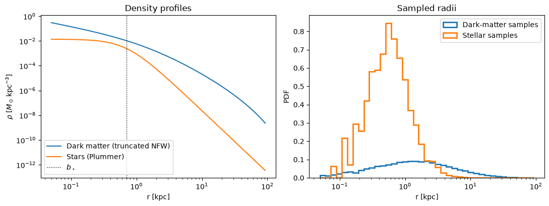
Because the stellar DF is computed in the combined potential, the stellar kinematics reflect the dark matter that dominates the mass budget. The dark matter inflates the stellar velocity dispersion well above what the stars’ self-gravity alone would produce — this is exactly the dynamical signature used to infer that dwarf spheroidals are dark-matter dominated.
Both examples above used isotropic DFs (eddingtondf), but the same recipe — build a DF in the (combined) potential and call sample — applies to the anisotropic DFs described below (e.g. the constant-\(\beta\) and Osipkov–Merritt models): just swap eddingtondf for the desired anisotropic DF class to give the sampled populations radially or tangentially biased velocity distributions.
[19]:
# Stellar radial velocity dispersion in the combined potential
sigma_with_dm = numpy.std(star_samples.vr())

# For comparison: the same stars in equilibrium with only their own gravity
df_st_nodm = eddingtondf(pot=stars, denspot=stars, rmax=3.0 * rvir_dw)
star_nodm = df_st_nodm.sample(n=n_star)
sigma_no_dm = numpy.std(star_nodm.vr())

print(f"Stellar sigma_r with dark matter:    {sigma_with_dm:.1f} km/s")
print(f"Stellar sigma_r from stars alone:    {sigma_no_dm:.1f} km/s")
Stellar sigma_r with dark matter:    8.8 km/s
Stellar sigma_r from stars alone:    3.5 km/s
Anisotropic DFs
galpy includes anisotropic DFs for spherical systems.
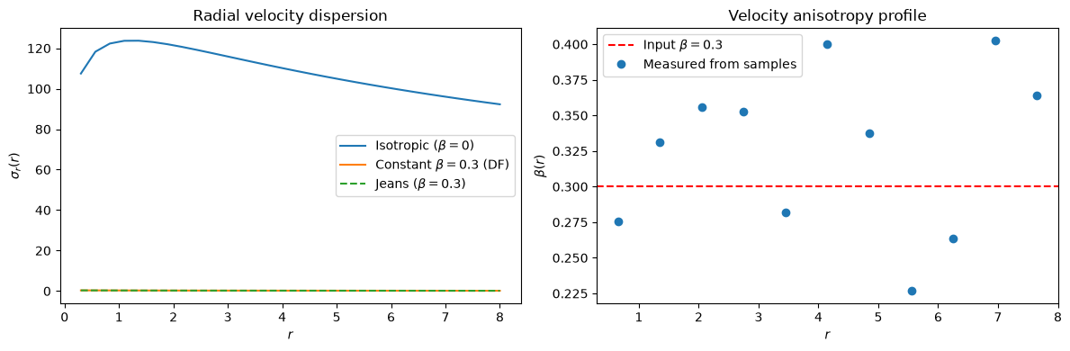
Constant-beta Hernquist DF
The constantbetaHernquistdf implements a Hernquist DF with constant velocity anisotropy parameter \(\beta\). Unlike the isotropic case (\(\beta=0\)), this DF has different radial and tangential velocity dispersions. The anisotropy parameter is defined as \(\beta = 1 - \sigma_t^2 / (2\sigma_r^2)\), so \(\beta > 0\) corresponds to radially-biased orbits and \(\beta < 0\) to tangentially-biased orbits.
[20]:
numpy.random.seed(1)
from galpy.df import constantbetaHernquistdf

hp = HernquistPotential(amp=2.0, a=1.3)
dfb = constantbetaHernquistdf(pot=hp, beta=0.3)

# Sample and compute the velocity anisotropy from samples
samples_b = dfb.sample(n=10000)
r_b = samples_b.r()
vr_b = samples_b.vr()
vt2_b = samples_b.vx() ** 2 + samples_b.vy() ** 2 + samples_b.vz() ** 2 - vr_b**2

# Compare analytical sigma_r with isotropic and Jeans equation
rs = numpy.linspace(0.3, 8.0, 30)
sigmar_beta = numpy.array([dfb.sigmar(r) for r in rs])
sigmar_iso = numpy.array([dfh.sigmar(r) for r in rs])
sigmar_jeans_beta = numpy.array(
    [jeans.sigmar(hp, r, beta=0.3, use_physical=False) for r in rs]
)

fig, axes = plt.subplots(1, 2, figsize=(12, 4))

# Left panel: velocity dispersion comparison
axes[0].plot(rs, sigmar_iso, label=r"Isotropic ($\beta=0$)")
axes[0].plot(rs, sigmar_beta, label=r"Constant $\beta=0.3$ (DF)")
axes[0].plot(rs, sigmar_jeans_beta, "--", label=r"Jeans ($\beta=0.3$)")
axes[0].set_xlabel(r"$r$")
axes[0].set_ylabel(r"$\sigma_r(r)$")
axes[0].legend()
axes[0].set_title("Radial velocity dispersion")

# Right panel: measured anisotropy from samples
rbins = numpy.linspace(0.3, 8.0, 12)
rmid = 0.5 * (rbins[:-1] + rbins[1:])
beta_measured = numpy.zeros(len(rmid))
for i in range(len(rmid)):
    mask = (r_b >= rbins[i]) & (r_b < rbins[i + 1])
    if numpy.sum(mask) > 10:
        sig_r2 = numpy.var(vr_b[mask])
        sig_t2 = numpy.mean(vt2_b[mask])
        beta_measured[i] = 1.0 - sig_t2 / (2.0 * sig_r2)

axes[1].axhline(0.3, color="r", ls="--", label=r"Input $\beta=0.3$")
axes[1].plot(rmid, beta_measured, "o", label="Measured from samples")
axes[1].set_xlabel(r"$r$")
axes[1].set_ylabel(r"$\beta(r)$")
axes[1].legend()
axes[1].set_title("Velocity anisotropy profile")
fig.tight_layout();
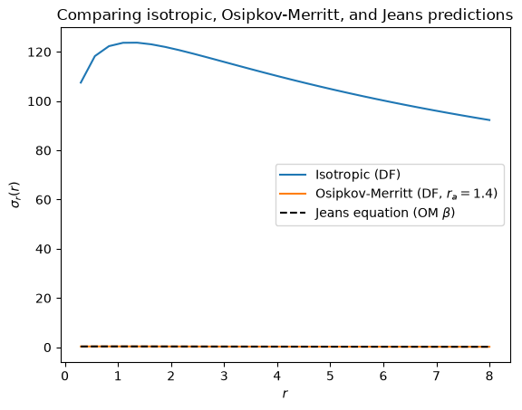
Osipkov-Merritt Hernquist DF
The Osipkov-Merritt DF is a widely used model for radially-anisotropic spherical systems. The velocity anisotropy varies with radius as \(\beta(r) = r^2/(r^2 + r_a^2)\), where \(r_a\) is the anisotropy radius. This means the system is nearly isotropic at the center (\(r \ll r_a\)) and becomes increasingly radially anisotropic at large radii (\(r \gg r_a\), \(\beta \to 1\)). Smaller values of \(r_a\) lead to stronger overall anisotropy.
[21]:
from galpy.df import osipkovmerrittHernquistdf

dfom = osipkovmerrittHernquistdf(pot=hp, ra=1.4)

# Compare velocity dispersion profiles: DF vs. Jeans equation
rs = numpy.linspace(0.3, 8.0, 30)
sig_iso = numpy.array([dfh.sigmar(r) for r in rs])
sig_om = numpy.array([dfom.sigmar(r) for r in rs])

# Jeans equation prediction with the OM beta profile
beta_om = lambda r: r**2 / (r**2 + 1.4**2)
sigmar_jeans_om = numpy.array(
    [jeans.sigmar(hp, r, beta=beta_om, use_physical=False) for r in rs]
)

plt.plot(rs, sig_iso, label="Isotropic (DF)")
plt.plot(rs, sig_om, label="Osipkov-Merritt (DF, $r_a=1.4$)")
plt.plot(rs, sigmar_jeans_om, "k--", label="Jeans equation (OM $\\beta$)")
plt.xlabel(r"$r$")
plt.ylabel(r"$\sigma_r(r)$")
plt.legend()
plt.title("Comparing isotropic, Osipkov-Merritt, and Jeans predictions");
For all anisotropic DFs, the sampling and evaluation methods work similarly to the isotropic case, but the velocity distribution will reflect the specified anisotropy.
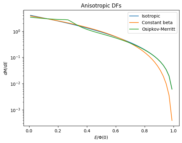
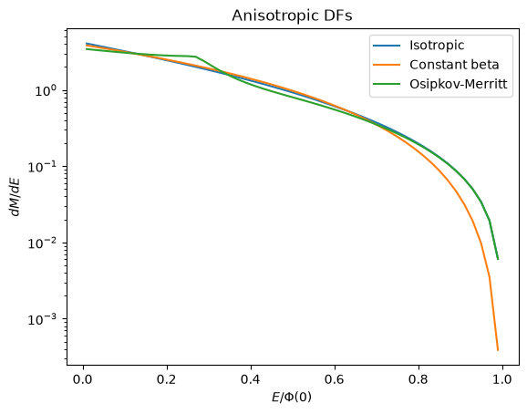
We can also compute the differential energy distribution for anisotropic DFs, which will differ from the isotropic case due to the different velocity structure.
[22]:
hp = HernquistPotential(amp=2.0, a=1.3)
dfh = isotropicHernquistdf(pot=hp)
dfh_constantbeta = constantbetaHernquistdf(pot=hp, beta=0.5)
dfh_ombeta = osipkovmerrittHernquistdf(pot=hp, ra=1.4)
# Evaluate at several energies
Es = numpy.linspace(0.01, 0.99, 50)
# Scale by Phi(0) to get the DF as a function of energy
phi0_hp = hp(0.0, 0.0, use_physical=False)
dMdE_hp = numpy.array([dfh.dMdE(E * phi0_hp) for E in Es])
dMdE_constantbeta = numpy.array([dfh_constantbeta.dMdE(E * phi0_hp) for E in Es])
dMdE_ombeta = numpy.array([dfh_ombeta.dMdE(E * phi0_hp) for E in Es])
plt.semilogy(Es, dMdE_hp, label="Isotropic")
plt.semilogy(Es, dMdE_constantbeta, label="Constant beta")
plt.semilogy(Es, dMdE_ombeta, label="Osipkov-Merritt")
plt.xlabel(r"$E / \Phi(0)$")
plt.ylabel(r"$dM/dE$")
plt.title("Anisotropic DFs")
plt.legend();
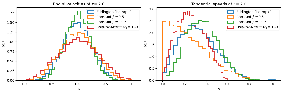
General formulas for computing constant-ansisotropy and Osipkov-Merritt DFs for any spherical potential are also implemented in the constantbetadf and osipkovmerrittdf classes, which can be used to compute the DF for any spherical potential with the specified anisotropy profile. For example, again embedding a Hernquist population in an NFW potential, we can compute the constant-beta and Osipkov-Merritt DFs for this system as follows and sample the different DFs to compare their velocity
distributions:
[23]:
from galpy.df import constantbetadf, osipkovmerrittdf

r0 = 2.0
n_samples = 8000
numpy.random.seed(1)

nfp = NFWPotential(amp=1.0, a=1.0)
hp = HernquistPotential(amp=2.0, a=1.3)
df_edd = eddingtondf(pot=nfp, denspot=hp)
# Use half-integer beta, for which the numerics are much faster
df_constb = constantbetadf(pot=nfp, denspot=hp, twobeta=1)
df_constb_low = constantbetadf(pot=nfp, denspot=hp, twobeta=-1)
df_omb = osipkovmerrittdf(pot=nfp, denspot=hp, ra=1.4)

samples_edd = df_edd.sample(n=n_samples, R=r0, z=0.0)
samples_constb = df_constb.sample(n=n_samples, R=r0, z=0.0)
samples_constb_low = df_constb_low.sample(n=n_samples, R=r0, z=0.0)
samples_omb = df_omb.sample(n=n_samples, R=r0, z=0.0)

vr_edd = samples_edd.vr()
vr_constb = samples_constb.vr()
vr_constb_low = samples_constb_low.vr()
vr_omb = samples_omb.vr()

vt_edd = numpy.sqrt(samples_edd.vT() ** 2 + samples_edd.vtheta() ** 2)
vt_constb = numpy.sqrt(samples_constb.vT() ** 2 + samples_constb.vtheta() ** 2)
vt_constb_low = numpy.sqrt(
    samples_constb_low.vT() ** 2 + samples_constb_low.vtheta() ** 2
)
vt_omb = numpy.sqrt(samples_omb.vT() ** 2 + samples_omb.vtheta() ** 2)

fig_vel, ax_vel = plt.subplots(1, 2, figsize=(12, 4))

ax_vel[0].hist(
    vr_edd, bins=31, density=True, histtype="step", lw=2, label="Eddington (isotropic)"
)
ax_vel[0].hist(
    vr_constb,
    bins=31,
    density=True,
    histtype="step",
    lw=2,
    label=r"Constant $\beta=0.5$",
)
ax_vel[0].hist(
    vr_constb_low,
    bins=31,
    density=True,
    histtype="step",
    lw=2,
    label=r"Constant $\beta=-0.5$",
)
ax_vel[0].hist(
    vr_omb,
    bins=31,
    density=True,
    histtype="step",
    lw=2,
    label=r"Osipkov-Merritt ($r_a=1.4$)",
)
ax_vel[0].set_xlabel(r"$v_r$")
ax_vel[0].set_ylabel("PDF")
ax_vel[0].set_title(rf"Radial velocities at $r={r0}$")
ax_vel[0].legend()

ax_vel[1].hist(
    vt_edd, bins=31, density=True, histtype="step", lw=2, label="Eddington (isotropic)"
)
ax_vel[1].hist(
    vt_constb,
    bins=31,
    density=True,
    histtype="step",
    lw=2,
    label=r"Constant $\beta=0.5$",
)
ax_vel[1].hist(
    vt_constb_low,
    bins=31,
    density=True,
    histtype="step",
    lw=2,
    label=r"Constant $\beta=-0.5$",
)
ax_vel[1].hist(
    vt_omb,
    bins=31,
    density=True,
    histtype="step",
    lw=2,
    label=r"Osipkov-Merritt ($r_a=1.4$)",
)
ax_vel[1].set_xlabel(r"$v_t$")
ax_vel[1].set_ylabel("PDF")
ax_vel[1].set_title(rf"Tangential speeds at $r={r0}$")
ax_vel[1].legend()

fig_vel.tight_layout();
Note that the calculation of constant-anisotropy DFs in this way requires the jax library to be installed, as it relies on automatic differentiation to compute the necessary derivatives of the potential and density profiles. The Osipkov-Merritt DFs can be computed without jax. Both can be quite slow.