This page was generated from a Jupyter notebook. You can download it here.
Phase-Space Volumes and Chaos
In addition to integrating orbits, galpy can integrate the variational equations: the linearized equations of motion that govern how an infinitesimal phase-space displacement \(\delta x\) evolves along an orbit. This is done with the Orbit.integrate_dxdv method, which works for two-dimensional (planar) and, since version 1.12, fully three-dimensional orbits, and is implemented in C for most potentials for speed.
Integrating deviation vectors gives access to the state-transition matrix \(M(t) = \partial x(t)/\partial x(0)\), whose columns are the evolved phase-space basis deviations. This allows you to
verify Liouville’s theorem (\(\det M = 1\): phase-space volume is conserved),
quantify the sensitivity of an orbit to its initial conditions, and
compute Lyapunov exponents to detect chaos, using the
Orbit.lyapunovmethod built on top ofintegrate_dxdv.
This tutorial briefly demonstrates each of these.
[1]:
%matplotlib inline
import matplotlib.pyplot as plt
import numpy

from galpy.orbit import Orbit
from galpy.potential import (
    HenonHeilesPotential,
    MWPotential2014,
    toPlanarPotential,
    toVerticalPotential,
)
Integrating phase-space deviations in 2D
For a planar orbit, the phase-space deviation is the four-vector \(\delta x = (\delta x, \delta y, \delta v_x, \delta v_y)\) in rectangular coordinates (use rectIn=True/rectOut=True to work entirely in this basis; otherwise galpy converts from/to cylindrical deviations). integrate_dxdv propagates the deviation with the linearized dynamics along the orbit; the deviation as a function of time is accessed with getOrbit_dxdv.
Integrating the four basis deviations builds up the state-transition matrix \(M(t)\), and Liouville’s theorem says that \(\det M(t) = 1\) at all times:
[2]:
mw2d = toPlanarPotential(MWPotential2014)
ts = numpy.linspace(0.0, 100.0, 1001)
M = numpy.empty((len(ts), 4, 4))
for ii in range(4):
    dxdv = numpy.zeros(4)
    dxdv[ii] = 1.0
    o = Orbit([1.0, 0.1, 1.1, 0.0])
    o.integrate_dxdv(dxdv, ts, mw2d, method="dop853_c", rectIn=True, rectOut=True)
    M[:, :, ii] = o.getOrbit_dxdv()
detM = numpy.linalg.det(M)
plt.semilogy(ts, numpy.fabs(detM - 1.0))
plt.xlabel(r"$t$")
plt.ylabel(r"$|\det M(t) - 1|$")
print(f"max |det M - 1| = {numpy.amax(numpy.fabs(detM - 1.0)):.2g}")
max |det M - 1| = 7.5e-07
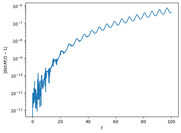
Phase-space volume is conserved to high precision (set by the integration tolerances) over the whole integration.
… and in 3D
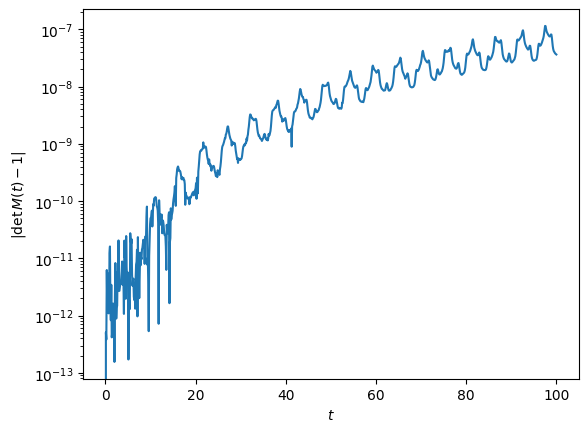
For three-dimensional orbits, everything works the same with the six-vector \(\delta x = (\delta x, \delta y, \delta z, \delta v_x, \delta v_y, \delta v_z)\) and the \(6\times6\) state-transition matrix; the full 3D Hessian of the potential is implemented in C for most potentials:
[3]:
ts = numpy.linspace(0.0, 100.0, 1001)
M = numpy.empty((len(ts), 6, 6))
for ii in range(6):
    dxdv = numpy.zeros(6)
    dxdv[ii] = 1.0
    o = Orbit([1.0, 0.1, 1.1, 0.0, 0.1, 0.0])
    o.integrate_dxdv(
        dxdv,
        ts,
        MWPotential2014,
        method="dop853_c",
        rectIn=True,
        rectOut=True,
        rtol=1e-12,
        atol=1e-12,
    )
    M[:, :, ii] = o.getOrbit_dxdv()
detM = numpy.linalg.det(M)
plt.semilogy(ts, numpy.fabs(detM - 1.0))
plt.xlabel(r"$t$")
plt.ylabel(r"$|\det M(t) - 1|$")
print(f"max |det M - 1| = {numpy.amax(numpy.fabs(detM - 1.0)):.2g}")
max |det M - 1| = 1.1e-07
… and in 1D
The variational equations are not limited to planar and three-dimensional orbits: they also work for one-dimensional (linear) orbits. A 1D orbit is created as Orbit([x, v]) and integrated in a linear potential — here the vertical motion of a star at the solar radius, obtained by freezing MWPotential2014 at \(R = 1\) with toVerticalPotential. The phase-space deviation is then simply the two-vector \(\delta x = (\delta x, \delta v)\) (there is no cylindrical-to-rectangular
conversion in 1D), the state-transition matrix is \(2\times2\), and once more \(\det M(t) = 1\):
[4]:
vp = toVerticalPotential(MWPotential2014, 1.0)
ts = numpy.linspace(0.0, 100.0, 1001)
M = numpy.empty((len(ts), 2, 2))
for ii in range(2):
    dxdv = numpy.zeros(2)
    dxdv[ii] = 1.0
    o = Orbit([0.1, 0.05])
    o.integrate_dxdv(dxdv, ts, vp, method="dop853_c")
    M[:, :, ii] = o.getOrbit_dxdv()
detM = numpy.linalg.det(M)
plt.semilogy(ts, numpy.fabs(detM - 1.0))
plt.xlabel(r"$t$")
plt.ylabel(r"$|\det M(t) - 1|$")
print(f"max |det M - 1| = {numpy.amax(numpy.fabs(detM - 1.0)):.2g}")
max |det M - 1| = 2.6e-08
Symplectic integration
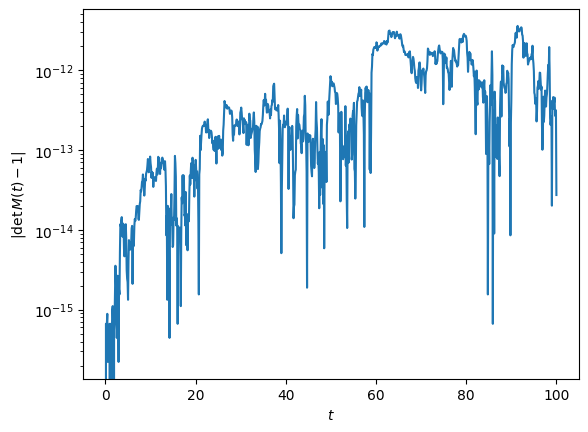
Every example so far used the high-order Runge–Kutta integrator dop853_c, but integrate_dxdv also supports galpy’s symplectic integrators — leapfrog_c, symplec4_c, and symplec6_c — in any dimension. Rather than integrating the variational right-hand side, these carry the deviation through the exact drift/kick tangent maps of each discrete step, so every step is symplectic by construction and the state-transition matrix conserves the symplectic form (and hence phase-space
volume) especially well. Symplectic integrators take a fixed step size dt. Repeating the planar example above with symplec4_c:
[5]:
ts = numpy.linspace(0.0, 100.0, 1001)
M = numpy.empty((len(ts), 4, 4))
for ii in range(4):
    dxdv = numpy.zeros(4)
    dxdv[ii] = 1.0
    o = Orbit([1.0, 0.1, 1.1, 0.0])
    o.integrate_dxdv(
        dxdv, ts, mw2d, method="symplec4_c", dt=0.01, rectIn=True, rectOut=True
    )
    M[:, :, ii] = o.getOrbit_dxdv()
detM = numpy.linalg.det(M)
plt.semilogy(ts, numpy.fabs(detM - 1.0))
plt.xlabel(r"$t$")
plt.ylabel(r"$|\det M(t) - 1|$")
print(f"max |det M - 1| = {numpy.amax(numpy.fabs(detM - 1.0)):.2g}")
max |det M - 1| = 3.6e-12
Lyapunov exponents and chaos
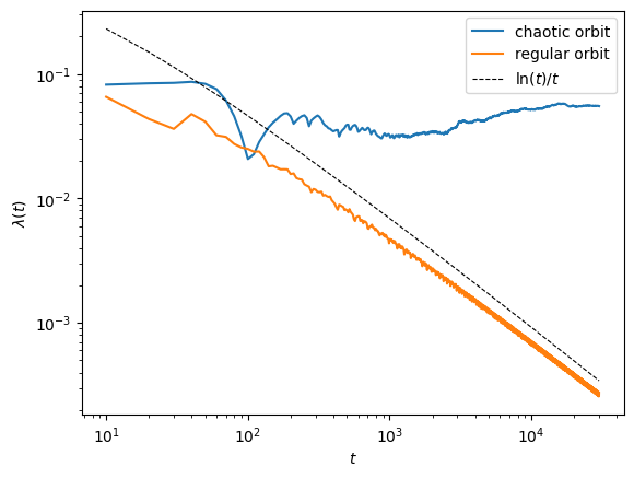
The growth rate of phase-space deviations is the classic diagnostic of chaos: for a regular orbit, deviations grow as a power of time, while for a chaotic orbit they grow exponentially, \(|\delta x(t)| \sim e^{\lambda t}\), with \(\lambda\) the largest Lyapunov exponent. Orbit.lyapunov estimates \(\lambda\) using the classic Benettin et al. (1980) method: it propagates a deviation vector with integrate_dxdv, renormalizes it regularly to avoid overflow, and accumulates the
growth factors into the running estimate \(\lambda(t)\), which is returned at all output times so that you can check its convergence. For a regular orbit, \(\lambda(t) \approx \ln(t)/t \rightarrow 0\), while for a chaotic orbit \(\lambda(t)\) converges to a positive value.
The Hénon–Heiles potential is the classic example of a system with a mix of regular and chaotic orbits. Here we compute the running Lyapunov estimate for a well-known chaotic and a well-known regular orbit at energy \(E = 1/8\) (orbits F and E of Skokos et al. 2002):
[6]:
hp = HenonHeilesPotential()
ts = numpy.linspace(0.0, 30000.0, 3001)
o_chaotic = Orbit([0.016, 0.0, 0.49974, -numpy.pi / 2.0])
lam_chaotic = o_chaotic.lyapunov(ts, pot=hp, method="dop853_c")
o_regular = Orbit([0.55, 0.0, -0.2417, numpy.pi / 2.0])
lam_regular = o_regular.lyapunov(ts, pot=hp, method="dop853_c")
plt.loglog(ts[1:], lam_chaotic[1:], label="chaotic orbit")
plt.loglog(ts[1:], lam_regular[1:], label="regular orbit")
plt.loglog(ts[1:], numpy.log(ts[1:]) / ts[1:], "k--", lw=0.8, label=r"$\ln(t)/t$")
plt.xlabel(r"$t$")
plt.ylabel(r"$\lambda(t)$")
plt.legend()
print(f"chaotic:  lambda = {lam_chaotic[-1]:.3f}")
print(f"regular:  lambda = {lam_regular[-1]:.2g}")
chaotic:  lambda = 0.055
regular:  lambda = 0.00027

The chaotic orbit’s estimate converges to \(\lambda \approx 0.05\) (consistent with the literature value for this orbit, e.g., Benettin et al. 1976), while the regular orbit’s estimate decays as \(\ln(t)/t\), the signature of regularity.
lyapunov works for three-dimensional orbits in the same way and supports physical outputs: when the orbit and potential carry physical scales, the returned exponent is in \(\mathrm{Gyr}^{-1}\) (it is a frequency). For example, for a mildly perturbed disk orbit in MWPotential2014 (a regular orbit, so the estimate decays):
[7]:
o = Orbit([1.0, 0.1, 1.1, 0.0, 0.1, 0.0], ro=8.0, vo=220.0)
ts = numpy.linspace(0.0, 1000.0, 101)
lam = o.lyapunov(ts, pot=MWPotential2014, method="dop853_c", renorm_every=5)
print(f"lambda(t_mid) = {lam[len(ts) // 2]:.2f}, lambda(t_end) = {lam[-1]:.2f}")
print("(decreasing -> consistent with a regular orbit; convergence to zero")
print(" requires much longer integration times)")
lambda(t_mid) = 0.38, lambda(t_end) = 0.21
(decreasing -> consistent with a regular orbit; convergence to zero
 requires much longer integration times)
For more details, see the API documentation of Orbit.integrate_dxdv, Orbit.getOrbit_dxdv, and Orbit.lyapunov.