This page was generated from a Jupyter notebook. You can download it here.

Using galpy Potentials in Other Codes

galpy potentials can be exported to and used within several other stellar dynamics and N-body simulation frameworks.

import warnings

warnings.filterwarnings("ignore", category=FutureWarning)
import numpy
from galpy.potential import MiyamotoNagaiPotential, MWPotential2014

NEMO

NEMO is a toolbox for stellar dynamics. It provides programs for creating N-body realizations of galaxies, integrating their evolution, and analyzing the results. One of the most widely used programs within NEMO is gyrfalcON (Dehnen 2000, 2002), a fast, momentum-conserving N-body code.

galpy potentials can be used as external gravitational fields in NEMO programs such as gyrfalcON. Two methods make this easy:

• nemo_accname(): returns the NEMO acceleration name for the potential

• nemo_accpars(vo, ro): returns the NEMO acceleration parameters, where vo and ro are the velocity and distance scales in km/s and kpc

For a single potential:

mp = MiyamotoNagaiPotential(a=0.5, b=0.0375, normalize=1.0)
print(mp.nemo_accname())

MiyamotoNagai

print(mp.nemo_accpars(220.0, 8.0))

0,592617.1107469305,4.0,0.3

For a composite potential like MWPotential2014, these methods automatically combine the individual components:

print(MWPotential2014.nemo_accname())

PowSphwCut+MiyamotoNagai+NFW

print(MWPotential2014.nemo_accpars(220.0, 8.0))

0,1001.7912681044569,1.8,1.9#0,306770.4183858958,3.0,0.28#0,16.0,162.95824180864443

You could then use these in a gyrfalcON command like:

gyrfalcON in.nemo out.nemo tstop=200 eps=0.05 step=0.01 kmax=8 \
  accname=MiyamotoNagai+NFW+MiyamotoNagai \
  accpars=<output of nemo_accpars>

galpy also includes a custom NEMO potential PowSphwCut in the galpy/nemo/ directory, which can be compiled and used for potentials based on PowerSphericalPotentialwCutoff.

The following galpy potentials support NEMO export:

• MiyamotoNagaiPotential

• NFWPotential

• PowerSphericalPotentialwCutoff

• PlummerPotential

• MN3ExponentialDiskPotential

• LogarithmicHaloPotential

• Any list of supported potentials

AMUSE

AMUSE (the Astrophysical Multipurpose Software Environment) is a Python framework for astrophysical simulations that combines existing codes for gravitational dynamics, stellar evolution, hydrodynamics, and radiative transfer.

galpy potentials can be converted to an AMUSE-compatible representation using the to_amuse function:

from galpy.potential import to_amuse, MWPotential2014
mwp_amuse = to_amuse(MWPotential2014)

The to_amuse function accepts the following keyword arguments:

• ro=, vo=: distance and velocity scales for unit conversion (default to galpy defaults)

• t=: current time in AMUSE units (default: 0 Myr)

• tgalpy=: current time in galpy natural units (alternative to t=)

• reverse=: if True, reverse the sign of the potential (useful for certain AMUSE bridge configurations)

Here is a complete example of setting up a Plummer-sphere cluster and evolving its N-body dynamics using an AMUSE BHTree in the external MWPotential2014 potential is:

from amuse.lab import *
from amuse.couple import bridge
from amuse.datamodel import Particles
from galpy.potential import to_amuse, MWPotential2014
from galpy.util import plot as galpy_plot

# Convert galpy MWPotential2014 to AMUSE representation
mwp_amuse= to_amuse(MWPotential2014)

# Set initial cluster parameters
N= 1000
Mcluster= 1000. | units.MSun
Rcluster= 10. | units.parsec
Rinit= [10.,0.,0.] | units.kpc
Vinit= [0.,220.,0.] | units.km/units.s
# Setup star cluster simulation
tend= 100.0 | units.Myr
dtout= 5.0 | units.Myr
dt= 1.0 | units.Myr

def setup_cluster(N,Mcluster,Rcluster,Rinit,Vinit):
    converter= nbody_system.nbody_to_si(Mcluster,Rcluster)
    stars= new_plummer_sphere(N,converter)
    stars.x+= Rinit[0]
    stars.y+= Rinit[1]
    stars.z+= Rinit[2]
    stars.vx+= Vinit[0]
    stars.vy+= Vinit[1]
    stars.vz+= Vinit[2]
    return stars,converter

# Setup cluster
stars,converter= setup_cluster(N,Mcluster,Rcluster,Rinit,Vinit)
cluster_code= BHTree(converter,number_of_workers=1) #Change number of workers depending no. of CPUs
cluster_code.parameters.epsilon_squared= (3. | units.parsec)**2
cluster_code.parameters.opening_angle= 0.6
cluster_code.parameters.timestep= dt
cluster_code.particles.add_particles(stars)

# Setup channels between stars particle dataset and the cluster code
channel_from_stars_to_cluster_code= stars.new_channel_to(cluster_code.particles,
                                       attributes=["mass", "x", "y", "z", "vx", "vy", "vz"])
channel_from_cluster_code_to_stars= cluster_code.particles.new_channel_to(stars,
                                       attributes=["mass", "x", "y", "z", "vx", "vy", "vz"])

# Setup gravity bridge
gravity= bridge.Bridge(use_threading=False)
# Stars in cluster_code depend on gravity from external potential mwp_amuse (i.e., MWPotential2014)
gravity.add_system(cluster_code, (mwp_amuse,))
# External potential mwp_amuse still needs to be added to system so it evolves with time
gravity.add_system(mwp_amuse,)
# Set how often to update external potential
gravity.timestep= cluster_code.parameters.timestep/2.
# Evolve
time= 0.0 | tend.unit
while time<tend:
    gravity.evolve_model(time+dt)
    # If you want to output or analyze the simulation, you need to copy
    # stars from cluster_code
    #channel_from_cluster_code_to_stars.copy()

    # If you edited the stars particle set, for example to remove stars from the
    # array because they have been kicked far from the cluster, you need to
    # copy the array back to cluster_code:
    #channel_from_stars_to_cluster_code.copy()

    # Update time
    time= gravity.model_time

channel_from_cluster_code_to_stars.copy()
gravity.stop()

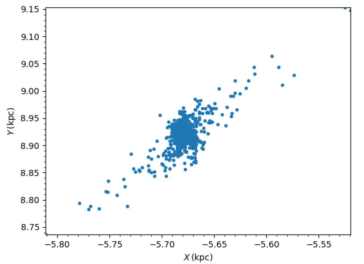
galpy_plot.plot(stars.x.value_in(units.kpc),stars.y.value_in(units.kpc),'.',
                    xlabel=r'$X\,(\mathrm{kpc})$',ylabel=r'$Y\,(\mathrm{kpc})$')

This should give a plot like the following, which shows a cluster in the first stages of disruption:

AGAMA

The AGAMA library (Action-based Galaxy Modelling Architecture) by Vasiliev (2019) supports importing galpy potentials. See the AGAMA documentation for details.

gala

The gala package by Price-Whelan (2017) supports converting galpy potentials. See the gala documentation for details on interoperability.