This page was generated from a Jupyter notebook. You can download it here.

SCF and Multipole Expansions

galpy supports two complementary basis-function-expansion techniques for representing the gravitational potential of arbitrary density distributions:

• SCFPotential uses the self-consistent field (SCF) method of Hernquist & Ostriker (1992), which expands a density in a biorthogonal basis set built from the Hernquist potential. This works well for smooth, roughly spheroidal systems.

• MultipoleExpansionPotential uses a spherical-harmonic (multipole) expansion where the radial functions are computed by direct integration. This is often more accurate than SCF for non-spherical systems, and it naturally supports time dependence.

For background on multipole expansions, see Chapter 12.3.1 of Bovy (2026). The SCF method is based on Hernquist & Ostriker (1992).

Both approaches let you turn any density function into a potential that can be used for orbit integration, action-angle calculations, and all other galpy operations. This tutorial demonstrates how to use both, and also covers the disk-specific variants DiskSCFPotential and DiskMultipoleExpansionPotential.

%matplotlib inline
import warnings

warnings.filterwarnings("ignore", category=RuntimeWarning)
warnings.filterwarnings("ignore", category=UserWarning)
import numpy
from matplotlib import pyplot as plt
from galpy import potential
from galpy.potential import (
    SCFPotential,
    MultipoleExpansionPotential,
    DiskSCFPotential,
    TriaxialNFWPotential,
    SolidBodyRotationWrapperPotential,
    HernquistPotential,
    DoubleExponentialDiskPotential,
    scf_compute_coeffs_spherical,
)
from galpy.orbit import Orbit

SCFPotential from a density

The SCFPotential.from_density class method builds an SCF expansion from any density function. As an example, we use a TriaxialNFWPotential with c=1.4, which stretches the density along the \(z\)-axis and makes the isodensity surfaces oblate (flattened in \(R\)). We use a large SCF scale length a=50 and expansion orders N=80, L=40.

tri_nfw = TriaxialNFWPotential(normalize=1.0, c=1.4, a=1.0)

scf_tri = SCFPotential.from_density(
    tri_nfw.dens, 80, L=40, a=50.0, symmetry="axisymmetry"
)

Here symmetry='axisymmetry' indicates that we are assuming axisymmetry in the basis-function expansion; other valid values are symmetry='spherical' when assuming spherical symmetry or symmetry=None for the general, non-axisymmetric computation.

We can check how well the SCF expansion reproduces the true density by comparing along the \(R = z\) line:

xs = numpy.linspace(0.01, 3.0, 1001)
plt.loglog(xs, [tri_nfw.dens(x, x) for x in xs], label="True density")
plt.loglog(xs, scf_tri.dens(xs, xs), "--", label="SCF expansion")
plt.xlabel(r"$R = z$")
plt.ylabel(r"Density")
plt.legend(frameon=False)
plt.title("TriaxialNFW: SCF density comparison along R = z");

The SCF expansion matches the true density very well over several orders of magnitude.

MultipoleExpansionPotential from a density

MultipoleExpansionPotential.from_density provides an alternative expansion using spherical harmonics. We build one for the same oblate TriaxialNFW density.

Tip

Because MultipoleExpansionPotential supports time-dependent densities, it checks whether the density function accepts a t parameter. If you pass a method like tri_nfw.dens (which has a t keyword), it will be interpreted as time-dependent and require a tgrid. To avoid this, pass the potential object directly (as below) or wrap the density in a lambda that strips the t parameter: lambda R, z, phi: pot.dens(R, z, phi).

mep_tri = MultipoleExpansionPotential.from_density(
    tri_nfw, L=40, symmetry="axisymmetry"
)

Now we can compare all three densities (true, SCF, and multipole) in a single plot:

xs = numpy.linspace(0.01, 3.0, 1001)
plt.loglog(xs, [tri_nfw.dens(x, x) for x in xs], label="True density")
plt.loglog(xs, scf_tri.dens(xs, xs), "--", label="SCF expansion")
plt.loglog(xs, mep_tri.dens(xs, xs), ":", label="Multipole expansion")
plt.xlabel(r"$R = z$")
plt.ylabel(r"Density")
plt.legend(frameon=False)
plt.title("True vs. SCF vs. Multipole density along R = z");

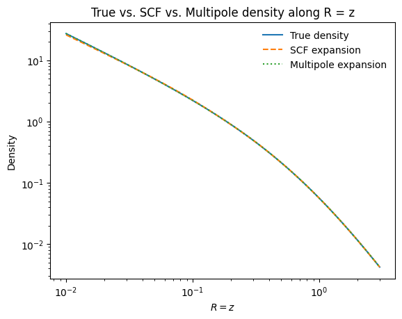
Both expansion methods faithfully reproduce the gravitational field and can be used for orbit integration, action-angle calculations, and all other galpy operations.

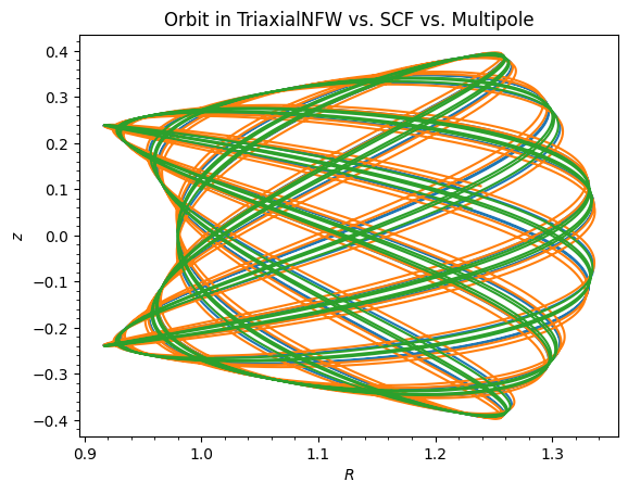
For example, we can integrate an orbit in the SCFPotential approximation to the triaxial NFW potential and compare it to the orbit in the true potential:

o = Orbit([1.0, 0.1, 1.1, 0.1, 0.3, 0.0])
ts = numpy.linspace(0.0, 100.0, 10001)
o.integrate(ts, tri_nfw)
o.plot()
o.integrate(ts, scf_tri)
o.plot(overplot=True)
o.integrate(ts, mep_tri)
o.plot(overplot=True)
plt.title("Orbit in TriaxialNFW vs. SCF vs. Multipole");

SCFPotential from an N-body representation

An SCFPotential can also be built directly from a set of particles — for example a snapshot from an N-body simulation — with SCFPotential.from_nbody, the N-body analogue of from_density. It takes the particle positions (pos, of shape [3,n] in rectangular coordinates) and their masses and evaluates the expansion coefficients as a direct sum over the particles. The sum is accumulated in batches, so building from a very large number of particles stays memory-bounded.

To illustrate this, we draw an isotropic sample from a spherical NFW halo with isotropicNFWdf, build an SCFPotential from the samples, and compare its rotation curve to a from_density build (the “direct” calculation) and to the exact result. Because isotropicNFWdf samples the halo out to a finite truncation radius rmax, we build from_density from the same density truncated at rmax, so the two represent the same mass distribution. We compare the circular velocity rather than the density because, like any basis-function expansion truncated at a modest order, the SCF reproduces the potential and forces of a cuspy NFW profile much more accurately than its density; representing the full, formally infinite-mass NFW this well would require a larger N.

from galpy.df import isotropicNFWdf

nfw = potential.NFWPotential(amp=1.0, a=2.0)
nfw.turn_physical_off()
rmax = 100.0
nfw_df = isotropicNFWdf(nfw, rmax=rmax)
numpy.random.seed(42)
n = 300_000
samples = nfw_df.sample(n=n)
pos = numpy.array([samples.x(), samples.y(), samples.z()])
# per-particle mass, so the sampled particles reproduce the halo's mass profile
mass = nfw.mass(rmax, use_physical=False) / n


# the sample is truncated at rmax, so for a fair, like-for-like comparison we build
# from_density from the *same* density truncated at rmax
def nfw_dens_truncated(R, z=0.0, phi=0.0):
    r = numpy.sqrt(R**2 + z**2)
    return nfw.dens(R, z, use_physical=False) * (r < rmax)


scf_nbody = SCFPotential.from_nbody(pos, N=15, symmetry="spherical", a=2.0, mass=mass)
scf_dens = SCFPotential.from_density(
    nfw_dens_truncated, N=15, symmetry="spherical", a=2.0
)

rs = numpy.linspace(0.2, 30.0, 100)
vc_true = numpy.array([nfw.vcirc(r, use_physical=False) for r in rs])
vc_dens = numpy.array([scf_dens.vcirc(r, use_physical=False) for r in rs])
vc_nbody = numpy.array([scf_nbody.vcirc(r, use_physical=False) for r in rs])

fig, axes = plt.subplots(1, 2, figsize=(9.5, 4.0))
axes[0].plot(rs, vc_true, "k-", lw=2.5, label="true NFW")
axes[0].plot(rs, vc_dens, "C0--", lw=2.0, label="SCF from_density")
axes[0].plot(rs, vc_nbody, "C1:", lw=2.5, label="SCF from_nbody")
axes[0].set_xlabel(r"$r$")
axes[0].set_ylabel(r"$v_c(r)$")
axes[0].legend()
axes[1].axhline(0.0, color="k", lw=1)
axes[1].plot(rs, vc_dens / vc_true - 1.0, "C0--", lw=2.0, label="from_density")
axes[1].plot(rs, vc_nbody / vc_true - 1.0, "C1:", lw=2.5, label="from_nbody")
axes[1].set_xlabel(r"$r$")
axes[1].set_ylabel(r"$v_c / v_{c,\mathrm{true}} - 1$")
axes[1].legend()
fig.tight_layout();

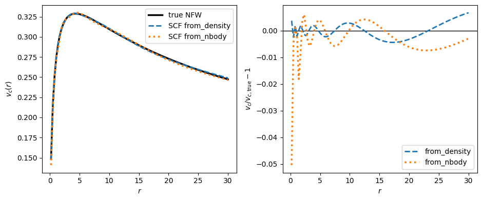
The SCF built from the particles closely tracks the one built from the smooth density; the small residual (right panel) is the Poisson noise of the finite sample, while the from_density build is smooth. As with from_density, passing multiple snapshots — pos of shape [3,n,nt] together with a tgrid of length nt — builds a time-dependent SCFPotential, with the coefficients computed at each snapshot and interpolated in time. This makes it easy to turn the output of an N-body simulation directly into a smooth, time-dependent potential.

Translating between the SCF and multipole expansions

Because the SCFPotential and MultipoleExpansionPotential both expand the density in the same real spherical harmonics, you can translate directly between them without going back to the density: MultipoleExpansionPotential.from_scf builds a multipole expansion from an SCF, and SCFPotential.from_multipole builds an SCF from a multipole expansion. Only the radial part is re-expanded — the angular decomposition is shared, so no angular quadrature is needed — and time-dependent expansions are translated as well.

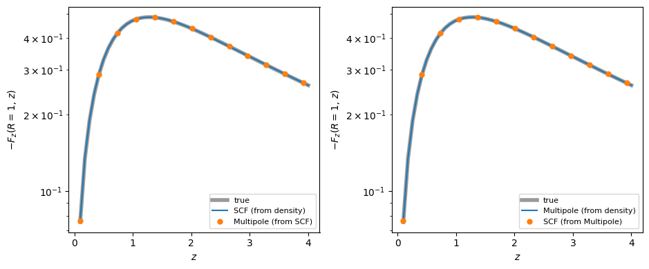
We build SCF and multipole expansions of the same triaxial NFW halo from the first section over a common radial range, translate each into the other representation, and confirm that the translations (markers) reproduce the independently-built expansions (lines) and the true vertical force:

# build SCF and multipole expansions of the same halo over a common radial range
rgrid = numpy.geomspace(1e-3, 200.0, 601)
scf_halo = SCFPotential.from_density(
    tri_nfw.dens, 40, L=20, a=50.0, symmetry="axisymmetry"
)
mep_halo = MultipoleExpansionPotential.from_density(
    tri_nfw, L=20, rgrid=rgrid, symmetry="axisymmetry"
)
# translate each expansion into the other representation
mep_from_scf = MultipoleExpansionPotential.from_scf(scf_halo, rgrid=rgrid)
scf_from_mep = SCFPotential.from_multipole(mep_halo, N=40, a=50.0)

zs = numpy.linspace(0.1, 4.0, 50)
Fz = lambda p, zv=zs: numpy.array([-p.zforce(1.0, z, use_physical=False) for z in zv])
zm = zs[::4]  # sparse points for the translated-expansion markers
fig, axes = plt.subplots(1, 2, figsize=(9.5, 4.0))
axes[0].plot(zs, Fz(tri_nfw), color="0.6", lw=4, label="true", zorder=1)
axes[0].plot(zs, Fz(scf_halo), "C0-", lw=1.5, label="SCF (from density)", zorder=2)
axes[0].plot(
    zm, Fz(mep_from_scf, zm), "C1o", ms=5, label="Multipole (from SCF)", zorder=3
)
axes[1].plot(zs, Fz(tri_nfw), color="0.6", lw=4, label="true", zorder=1)
axes[1].plot(
    zs, Fz(mep_halo), "C0-", lw=1.5, label="Multipole (from density)", zorder=2
)
axes[1].plot(
    zm, Fz(scf_from_mep, zm), "C1o", ms=5, label="SCF (from Multipole)", zorder=3
)
for ax in axes:
    ax.set_yscale("log")
    ax.set_xlabel(r"$z$")
    ax.set_ylabel(r"$-F_z(R=1,\,z)$")
    ax.legend(fontsize=8)
fig.tight_layout();

Computing SCF coefficients manually

Instead of using from_density, you can compute the SCF expansion coefficients yourself and pass them directly to SCFPotential. This is useful when you want to inspect the coefficients or store them for later use. The scf_compute_coeffs_spherical, scf_compute_coeffs_axi, and scf_compute_coeffs functions compute the coefficients from a density, while their scf_compute_coeffs_spherical_nbody, scf_compute_coeffs_axi_nbody, and scf_compute_coeffs_nbody counterparts do the same directly from an N-body particle set (as used by from_nbody above).

The Hernquist profile is the lowest-order SCF basis function, so only the zeroth-order coefficient should be non-zero in the following example:

hp = HernquistPotential(amp=1.0, a=2.0)
Acos, Asin = scf_compute_coeffs_spherical(hp.dens, 10, a=2.0)
print("Acos coefficients:")
print(Acos)
print(
    "\nAs expected, only Acos[0,0,0] = 1.0 is non-zero; all others are at machine precision."
)

Acos coefficients:
[[[ 1.00000000e+00]]

 [[ 8.65722568e-18]]

 [[-1.13278379e-16]]

 [[-2.93522527e-18]]

 [[-3.04900866e-17]]

 [[-8.03257697e-20]]

 [[-1.36005913e-17]]

 [[ 1.30909657e-18]]

 [[-5.31153122e-18]]

 [[-6.69176217e-19]]]

As expected, only Acos[0,0,0] = 1.0 is non-zero; all others are at machine precision.

To build an SCFPotential from these coefficients:

sp_hernquist = SCFPotential(Acos=Acos, Asin=Asin, a=2.0)
print(sp_hernquist)

SCFPotential with internal parameters: amp=0.5, Acos=[[[ 2.82094792e-01]]

 [[ 2.44215828e-18]]

 [[-3.19552407e-17]]

 [[-8.28011762e-19]]

 [[-8.60109462e-18]]

 [[-2.26594813e-20]]

 [[-3.83665598e-18]]

 [[ 3.69289325e-19]]

 [[-1.49835529e-18]]

 [[-1.88771125e-19]]], Asin=[[[0.]]

 [[0.]]

 [[0.]]

 [[0.]]

 [[0.]]

 [[0.]]

 [[0.]]

 [[0.]]

 [[0.]]

 [[0.]]], a=2.0 and physical outputs off

Note that the internally-stored coefficients are modified by the normalization factors of the basis functions, so they are not exactly the same as the input coefficients.

DiskSCFPotential

For disk-like density distributions, the standard SCF expansion converges slowly because spherical basis functions are a poor match for thin, flat structures. DiskSCFPotential uses a trick to greatly improve convergence for disky systems.

The disk density is approximated as \(\rho_{\mathrm{disk}}(R,\phi,z) \approx \sum_i \Sigma_i(R)\,h_i(z)\), with \(h_i(z) = \mathrm{d}^2 H(z) / \mathrm{d} z^2\), and the potential is written as

\[\Phi(R,\phi,z) = \Phi_{\mathrm{ME}}(R,\phi,z) + 4\pi G\sum_i \Sigma_i(r)\,H_i(z)\]

where \(r^2 = R^2+z^2\) is the spherical radius. The density giving rise to \(\Phi_{\mathrm{ME}}\) is not strongly confined to a plane and can be obtained using the multipole or SCF methods. This trick is due to Kuijken & Dubinski (1995).

As an example, we represent a DoubleExponentialDiskPotential with \(h_R = 1/3\) and \(h_z = 1/27\):

dp = DoubleExponentialDiskPotential(amp=13.5, hr=1.0 / 3.0, hz=1.0 / 27.0)

dscfp = DiskSCFPotential(
    dens=lambda R, z: dp.dens(R, z),
    Sigma={"type": "exp", "h": 1.0 / 3.0, "amp": 1.0},
    hz={"type": "exp", "h": 1.0 / 27.0},
    a=1.0,
    N=10,
    L=10,
)

Compare the density along the \(R = 10z\) line:

xs = numpy.linspace(0.3, 2.0, 1001)
plt.semilogy(xs, dp.dens(xs, xs / 10.0), label="DoubleExponentialDisk")
plt.semilogy(xs, dscfp.dens(xs, xs / 10.0), "--", label="DiskSCFPotential")
plt.xlabel(r"$R$")
plt.ylabel(r"Density")
plt.legend(frameon=False)
plt.title("Density along R = 10z");

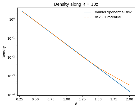
The DiskSCFPotential reproduces the disk density very well. Orbit integration in DiskSCFPotential is also much faster than in DoubleExponentialDiskPotential, because the latter requires expensive numerical integrals at every force evaluation whereas DiskSCFPotential evaluates analytic basis functions:

ts = numpy.linspace(0.0, 100.0, 10001)
ic_disk = [1.0, 0.1, 0.9, 0.0, 0.1, 0.0]

o_dscf = Orbit(ic_disk)
o_dscf.integrate(ts, dscfp)
o_dscf.plot()
o_dp = Orbit(ic_disk)
o_dp.integrate(ts, dp)
o_dp.plot(overplot=True)
plt.title("Orbit in DiskSCFPotential vs. DoubleExponentialDiskPotential");

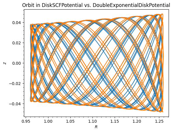
The orbits agree closely, but DiskSCFPotential is dramatically faster for orbit integration. Compare

%%timeit
o.integrate(ts, dp)
# 4.53 s ± 25.4 ms per loop (mean ± std. dev. of 7 runs, 1 loop each)

2.65 s ± 157 ms per loop (mean ± std. dev. of 7 runs, 1 loop each)

and

%%timeit
o.integrate(ts, dscfp)
# 57.2 ms ± 99.6 µs per loop (mean ± std. dev. of 7 runs, 10 loops each)

79.9 ms ± 548 μs per loop (mean ± std. dev. of 7 runs, 10 loops each)

DiskMultipoleExpansionPotential

galpy also provides DiskMultipoleExpansionPotential, which applies the same Kuijken & Dubinski disk-subtraction technique but uses a MultipoleExpansionPotential (instead of SCF) to solve the residual Poisson equation. Usage is analogous to DiskSCFPotential and can be more accurate for some density profiles.

Time-dependent MultipoleExpansionPotential

The MultipoleExpansionPotential supports time-dependent densities. If you pass a density function that accepts a t keyword argument together with a tgrid array, galpy precomputes the expansion at each time step and interpolates. This is most useful for modeling potentials with complex time dependence, e.g., a time-dependent shape. In the following, we use a rotating bar as a simple example, but note that adding simple rotation is most easily accomplished using existing (or new) wrappers.

As an example, we build a Hernquist-like density with a \(\cos(2\phi)\) bar perturbation rotating at pattern speed \(\Omega_p = 1.5\):

OmegaP = 1.5


def rotating_bar_dens(R, z, phi=0.0, t=0.0):
    phi_bar = phi - OmegaP * t
    r2 = R**2 + z**2
    rho0 = 1.0 / (r2**0.5 * (1.0 + r2**0.5) ** 3)
    return rho0 * (1.0 + 0.3 * numpy.cos(2.0 * phi_bar))


mep_td = MultipoleExpansionPotential.from_density(
    rotating_bar_dens,
    L=4,
    rgrid=numpy.geomspace(0.01, 20.0, 101),
    symmetry=None,
    tgrid=numpy.linspace(0.0, 4.0 * numpy.pi / OmegaP, 51),
)

We can visualize how the potential varies with azimuth at different times, confirming that the bar pattern rotates:

phis = numpy.linspace(0.0, 2.0 * numpy.pi, 100)
for t in [0.0, 1.0]:
    vals = [mep_td(1.0, 0.0, phi=phi, t=t) for phi in phis]
    plt.plot(phis, vals, label=f"t = {t:.1f}")
plt.xlabel(r"$\phi$")
plt.ylabel(r"$\Phi$")
plt.legend()
plt.title("Time-dependent multipole expansion: rotating bar");

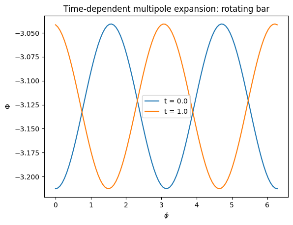
The phase shift between the two curves shows the bar rotating at the specified pattern speed. This time-dependent multipole expansion can be used for orbit integration in the same way as any other galpy potential. For example, we can integrate an orbit in a rotating bar-like perturbation on top of a Hernquist halo. First we build the combined potential:

hp = HernquistPotential(normalize=1.0, a=1.0)
omega = 1.3
epsilon = 0.125
tgrid = numpy.linspace(0, 60, 251)
mp_tdep = MultipoleExpansionPotential.from_density(
    lambda R, z, phi, t=0.0: (
        hp.dens(R, z, use_physical=False)
        * (1 + epsilon * numpy.cos(2 * (phi - omega * t)))
    ),
    L=4,
    rgrid=numpy.geomspace(1e-3, 30, 201),
    tgrid=tgrid,
)

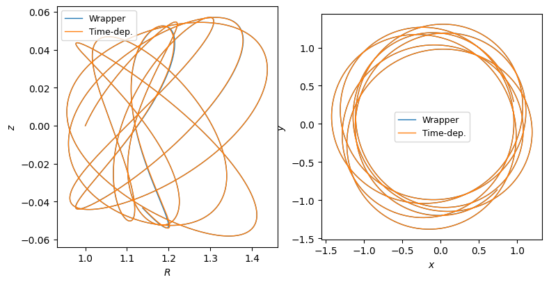
Then, we integrate an orbit in this potential and compare it to the equivalent SolidBodyRotationWrapperPotential approach:

mp_static = MultipoleExpansionPotential.from_density(
    lambda R, z, phi: (
        hp.dens(R, z, use_physical=False) * (1 + epsilon * numpy.cos(2 * phi))
    ),
    L=4,
    rgrid=numpy.geomspace(1e-3, 30, 201),
)
mp_wrapped = SolidBodyRotationWrapperPotential(pot=mp_static, omega=omega)
from galpy.orbit import Orbit

ts = numpy.linspace(0, 50, 5001)
o_wrap = Orbit([1.0, 0.1, 1.1, 0.0, 0.05, 0.3])
o_tdep = Orbit([1.0, 0.1, 1.1, 0.0, 0.05, 0.3])
o_wrap.integrate(ts, mp_wrapped)
o_tdep.integrate(ts, mp_tdep)

fig, axes = plt.subplots(1, 2, figsize=(9, 4.5))
axes[0].plot(o_wrap.R(ts), o_wrap.z(ts), lw=1.0, label="Wrapper")
axes[0].plot(o_tdep.R(ts), o_tdep.z(ts), lw=1.0, label="Time-dep.")
axes[0].set_xlabel(r"$R$")
axes[0].set_ylabel(r"$z$")
axes[0].legend(fontsize=9)
axes[1].plot(
    o_wrap.R(ts) * numpy.cos(o_wrap.phi(ts)),
    o_wrap.R(ts) * numpy.sin(o_wrap.phi(ts)),
    lw=1.0,
    label="Wrapper",
)
axes[1].plot(
    o_tdep.R(ts) * numpy.cos(o_tdep.phi(ts)),
    o_tdep.R(ts) * numpy.sin(o_tdep.phi(ts)),
    lw=1.0,
    label="Time-dep.",
)
axes[1].set_xlabel(r"$x$")
axes[1].set_ylabel(r"$y$")
axes[1].legend(fontsize=9)
axes[1].set_aspect("equal")

Time-dependent SCFPotential

The SCFPotential supports time-dependent densities in the same way as the MultipoleExpansionPotential: pass a density function that accepts a t keyword argument together with a tgrid array, and galpy computes the expansion coefficients at each time step and interpolates them in time with a cubic spline. (Equivalently, you can initialize an SCFPotential directly with time-dependent coefficients by passing Acos/Asin as callables f(t) returning the coefficient array, or as (Nt, N, L, M) arrays sampled on tgrid.) The potential, forces, second derivatives, and density are then evaluated efficiently — in both Python and C — at arbitrary times during orbit integration.

Tip

Unlike MultipoleExpansionPotential.from_density, SCFPotential.from_density treats the density as time-dependent only when a tgrid is passed; it does not otherwise inspect the density for a t parameter. So the footgun noted above for the multipole does not arise here: passing a method like tri_nfw.dens (which has a t keyword) without a tgrid simply builds the static potential.

The same physical caveats as for the time-dependent multipole apply: an astropy Quantity (physical-unit) density is not supported on the time-dependent path, so pass the density in galpy’s internal units. As for the multipole, the coefficient computation is vectorized over time — the time-independent basis functions are built once and the density is sampled at all times at once, a large speed-up over a per-time-step loop (a density that cannot be evaluated on an array of times falls back to that loop). Because the vectorized quadrature accumulates an array with a leading time axis, galpy processes the tgrid in memory-bounded batches internally, so peak memory stays bounded even for a large number of time steps; what grows with the number of steps is the build time (roughly linearly), not memory. Once built, SCF evaluation (e.g. orbit integration) is very fast — for a smooth density well matched to the SCF scale length, several times faster than the equivalent multipole.

To illustrate and validate the time dependence, we build a time-dependent SCFPotential and MultipoleExpansionPotential from the same rigidly rotating \(m=2\) bar density (a Hernquist halo with a \(\cos[2(\phi-\Omega_p t)]\) perturbation at pattern speed \(\Omega_p=1.3\)). Because the pattern rotates rigidly, its exact time-dependent potential is simply the static potential rotated — which galpy also builds directly with SolidBodyRotationWrapperPotential — giving us a reference to check each expansion against:

hp_bar = HernquistPotential(normalize=1.0, a=1.0)
OmegaP_bar = 1.3
T_bar = 2.0 * numpy.pi / OmegaP_bar  # rotation period
bar_tgrid = numpy.linspace(0.0, 2.0 * T_bar, 51)  # two rotation periods


def rotating_bar_density(R, z, phi=0.0, t=0.0):
    return hp_bar.dens(R, z, use_physical=False) * (
        1.0 + 0.2 * numpy.cos(2.0 * (phi - OmegaP_bar * t))
    )


def static_bar_density(R, z, phi):  # the t=0 snapshot
    return rotating_bar_density(R, z, phi, 0.0)


# Time-dependent SCF and multipole from the same rotating density. The SCF build
# is vectorized over time (and internally batched to bound memory); a modest
# angular quadrature is plenty for this smooth m=2 bar and keeps the build quick
scf_bar = SCFPotential.from_density(
    rotating_bar_density,
    N=8,
    L=3,
    symmetry=None,
    tgrid=bar_tgrid,
    costheta_order=10,
    phi_order=10,
)
mep_bar = MultipoleExpansionPotential.from_density(
    rotating_bar_density,
    L=3,
    rgrid=numpy.geomspace(1e-3, 30, 101),
    tgrid=bar_tgrid,
)
# The exact rigid rotation of each static expansion (SolidBodyRotationWrapper)
scf_wrapped = SolidBodyRotationWrapperPotential(
    pot=SCFPotential.from_density(static_bar_density, N=8, L=3, symmetry=None),
    omega=OmegaP_bar,
)
mep_wrapped = SolidBodyRotationWrapperPotential(
    pot=MultipoleExpansionPotential.from_density(
        static_bar_density, L=3, rgrid=numpy.geomspace(1e-3, 30, 101)
    ),
    omega=OmegaP_bar,
)

phis = numpy.linspace(0.0, 2.0 * numpy.pi, 200)
fig, axes = plt.subplots(1, 2, figsize=(9.5, 4.0))
# Left: the pattern rotates; time-dep SCF (solid) vs time-dep multipole (dashed)
for t, c in zip([0.0, T_bar / 8.0, T_bar / 4.0], ["C0", "C1", "C2"]):
    p_scf = numpy.array(
        [scf_bar(1.0, 0.0, phi=p, t=t, use_physical=False) for p in phis]
    )
    p_mep = numpy.array(
        [mep_bar(1.0, 0.0, phi=p, t=t, use_physical=False) for p in phis]
    )
    axes[0].plot(phis, p_mep, c + "--", lw=3.0, alpha=0.4)
    axes[0].plot(phis, p_scf, c + "-", lw=1.3, label=f"$t = {t:.2f}$")
axes[0].set_xlabel(r"$\phi$")
axes[0].set_ylabel(r"$\Phi(R=1,\,z=0,\,\phi,\,t)$")
axes[0].legend(fontsize=8, title="SCF (—) vs. Multipole (– –)")
# Right: each time-dep expansion vs its own solid-body-rotated static potential
t = T_bar / 8.0
r_scf = numpy.array(
    [
        scf_bar(1.0, 0.0, phi=p, t=t, use_physical=False)
        - scf_wrapped(1.0, 0.0, phi=p, t=t, use_physical=False)
        for p in phis
    ]
)
r_mep = numpy.array(
    [
        mep_bar(1.0, 0.0, phi=p, t=t, use_physical=False)
        - mep_wrapped(1.0, 0.0, phi=p, t=t, use_physical=False)
        for p in phis
    ]
)
axes[1].plot(phis, r_scf, "C0-", label="SCF $-$ SCF-wrapper")
axes[1].plot(phis, r_mep, "C1-", label="Multipole $-$ Mult-wrapper")
axes[1].set_xlabel(r"$\phi$")
axes[1].set_ylabel(r"$\Phi - \Phi_{\mathrm{wrapper}}$")
axes[1].legend(fontsize=8)
axes[1].set_title(rf"reproduction of the exact rotation ($t={t:.2f}$)")
fig.tight_layout();

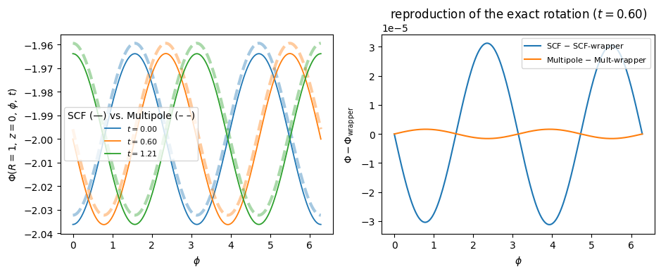
As the bar rotates, its \(m=2\) pattern sweeps around in \(\phi\) (left panel), and the time-dependent SCF (solid) and multipole (dashed) — two different expansions of the same density — agree to \(\sim10^{-3}\); that small offset is the ordinary truncation difference between the two bases (both converge as \(L\) increases), not a time-dependence effect. Indeed, each time-dependent expansion reproduces the exact rigid rotation of its own static expansion — the corresponding SolidBodyRotationWrapperPotential — to \(\sim10^{-5}\) (right panel), the cubic-spline-in-time interpolation error set by the density of tgrid. So the time-dependence itself is essentially exact; the SCF–multipole difference is purely about how each basis represents the truncated density. For a rigidly rotating pattern the wrapper is the simpler tool; the value of the time-dependent expansion is that it handles general time dependence, for which no such shortcut exists. 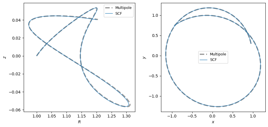Orbits integrated in the SCF and multipole expansions stay close over two bar rotations, with a small drift that reflects the same \(\sim10^{-3}\) truncation difference between the two bases, gradually accumulated by the orbit integration:

bar_ts = numpy.linspace(0.0, bar_tgrid[-1], 3001)
ic_bar = [1.0, 0.1, 1.1, 0.0, 0.05, 0.3]
o_scf = Orbit(ic_bar)
o_mep = Orbit(ic_bar)
o_scf.integrate(bar_ts, scf_bar)
o_mep.integrate(bar_ts, mep_bar)

fig, axes = plt.subplots(1, 2, figsize=(9.5, 4.5))
axes[0].plot(
    o_mep.R(bar_ts), o_mep.z(bar_ts), "k--", lw=3.0, alpha=0.4, label="Multipole"
)
axes[0].plot(o_scf.R(bar_ts), o_scf.z(bar_ts), "C0-", lw=1.0, label="SCF")
axes[0].set_xlabel(r"$R$")
axes[0].set_ylabel(r"$z$")
axes[0].legend(fontsize=9)
axes[1].plot(
    o_mep.R(bar_ts) * numpy.cos(o_mep.phi(bar_ts)),
    o_mep.R(bar_ts) * numpy.sin(o_mep.phi(bar_ts)),
    "k--",
    lw=3.0,
    alpha=0.4,
    label="Multipole",
)
axes[1].plot(
    o_scf.R(bar_ts) * numpy.cos(o_scf.phi(bar_ts)),
    o_scf.R(bar_ts) * numpy.sin(o_scf.phi(bar_ts)),
    "C0-",
    lw=1.0,
    label="SCF",
)
axes[1].set_xlabel(r"$x$")
axes[1].set_ylabel(r"$y$")
axes[1].legend(fontsize=9)
axes[1].set_aspect("equal")
fig.tight_layout();