Introduction

The most basic features of galpy are its ability to display rotation curves and perform orbit integration for arbitrary combinations of potentials. This section introduce the most basic features of galpy.potential and galpy.orbit.

Rotation curves

The following code example shows how to initialize a Miyamoto-Nagai disk potential and plot its rotation curve

>>> from galpy.potential import MiyamotoNagaiPotential
>>> mp= MiyamotoNagaiPotential(a=0.5,b=0.0375,normalize=1.)
>>> mp.plotRotcurve(Rrange=[0.01,10.],grid=1001)

The normalize=1. option normalizes the potential such that the radial force is a fraction normalize=1. of the radial force necessary to make the circular velocity 1 at R=1. Starting in v1.2 you can also initialize potentials with amplitudes and other parameters in physical units; see below and other parts of this documentation.

Tip

You can copy all of the code examples in this documentation to your clipboard by clicking the button in the top, right corner of each example. This can be directly pasted into a Python interpreter (including the >>>).

Similarly we can initialize other potentials and plot the combined rotation curve

>>> from galpy.potential import NFWPotential, HernquistPotential
>>> mp= MiyamotoNagaiPotential(a=0.5,b=0.0375,normalize=.6)
>>> np= NFWPotential(a=4.5,normalize=.35)
>>> hp= HernquistPotential(a=0.6/8,normalize=0.05)
>>> from galpy.potential import plotRotcurve
>>> plotRotcurve(hp+mp+np,Rrange=[0.01,10.],grid=1001,yrange=[0.,1.2])

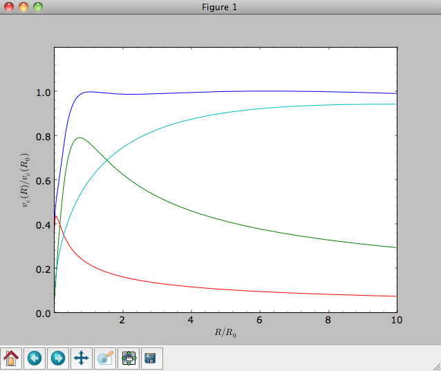
Note that the normalize values add up to 1. such that the circular velocity will be 1 at R=1. Potentials can be combined into a composite potential either by combining them in a list as [hp,mp,np] or by adding them up hp+mp+np (the latter simply returns the list [hp,mp,np]). The resulting rotation curve is approximately flat. To show the rotation curves of the three components do

>>> mp.plotRotcurve(Rrange=[0.01,10.],grid=1001,overplot=True)
>>> hp.plotRotcurve(Rrange=[0.01,10.],grid=1001,overplot=True)
>>> np.plotRotcurve(Rrange=[0.01,10.],grid=1001,overplot=True)

You’ll see the following

As a shortcut the [hp,mp,np] Milky-Way-like potential is defined as

>>> from galpy.potential import MWPotential

This is not the recommended Milky-Way-like potential in galpy. The (currently) recommended Milky-Way-like potential is MWPotential2014:

>>> from galpy.potential import MWPotential2014

MWPotential2014 has a more realistic bulge model and is actually fit to various dynamical constraints on the Milky Way (see here and the galpy paper).

Units in galpy

Internal (natural) units

Above we normalized the potentials such that they give a circular velocity of 1 at R=1. These are the standard galpy units (sometimes referred to as natural units in the documentation). galpy will work most robustly when using these natural units. When using galpy to model a real galaxy with, say, a circular velocity of 220 km/s at R=8 kpc, all of the velocities should be scaled as v= V/[220 km/s] and all of the positions should be scaled as x = X/[8 kpc] when using galpy’s natural units.

For convenience, a utility module conversion is included in galpy that helps in converting between physical units and natural units for various quantities. Alternatively, you can use the astropy units module to specify inputs in physical units and get outputs with units (see the next subsection below). For example, in natural units the orbital time of a circular orbit at R=1 is \(2\pi\); in physical units this corresponds to

>>> from galpy.util import conversion
>>> print(2.*numpy.pi*conversion.time_in_Gyr(220.,8.))
# 0.223405444283

or about 223 Myr. We can also express forces in various physical units. For example, for the Milky-Way-like potential defined in galpy, we have that the vertical force at 1.1 kpc is

>>> from galpy.potential import MWPotential2014, evaluatezforces
>>> -evaluatezforces(MWPotential2014, 1.,1.1/8.)*conversion.force_in_pcMyr2(220.,8.)
# 2.0259181908629933

which we can also express as an equivalent surface-density by dividing by \(2\pi G\)

>>> -evaluatezforces(MWPotential2014, 1.,1.1/8.)*conversion.force_in_2piGmsolpc2(220.,8.)
# 71.658016957792356

Because the vertical force at the solar circle in the Milky Way at 1.1 kpc above the plane is approximately \(70\,(2\pi G\, M_\odot\,\mathrm{pc}^{-2})\) (e.g., 2013arXiv1309.0809B), this shows that our Milky-Way-like potential has a realistic disk (at least in this respect).

conversion further has functions to convert densities, masses, surface densities, and frequencies to physical units (actions are considered to be too obvious to be included); see here for a full list. As a final example, the local dark matter density in the Milky-Way-like potential is given by

>>> MWPotential2014[2].dens(1.,0.)*conversion.dens_in_msolpc3(220.,8.)
# 0.0075419566970079373

or

>>> MWPotential2014[2].dens(1.,0.)*conversion.dens_in_gevcc(220.,8.)
# 0.28643101789044584

or about \(0.0075\,M_\odot\,\mathrm{pc}^{-3} \approx 0.3\,\mathrm{GeV\,cm}^{-3}\), in line with current measurements (e.g., 2012ApJ…756…89B).

When galpy Potentials, Orbits, actionAngles, or DFs are initialized using a distance scale ro= and a velocity scale vo= output quantities returned and plotted in physical coordinates. Specifically, positions are returned in the units in the table below. If astropy-units = True in the configuration file, then an astropy Quantity which includes the units is returned instead (see below).

Quantity	Default unit
position	kpc
velocity	km/s
angular velocity	km/s/kpc
energy	(km/s)^2
Jacobi integral	(km/s)^2
angular momentum	km/s x kpc
actions	km/s x kpc
frequencies	rad/Gyr
time	Gyr
period	Gyr
potential	(km/s)^2
force	km/s/Myr
force derivative	1/Gyr^2
density	Msun/pc^3
number density	1/pc^3
surface density	Msun/pc^2
mass	Msun
angle	rad
proper motion	mas/yr
phase-space density	1/(kpc x km/s)^3

Warning

When returned as a Quantity, frequencies get units of 1/Gyr, although in detail this means rad/Gyr (not cycles/Gyr).

Physical units

Tip

With astropy-units = True in the configuration file and specifying all inputs using astropy Quantity with units, galpy will return outputs in convenient, unambiguous units.

Full support for unitful quantities using astropy Quantity was added in v1.2. Thus, any input to a galpy Potential, Orbit, actionAngle, or DF instantiation, method, or function can now be specified in physical units as a Quantity. For example, we can set up a Miyamoto-Nagai disk potential with a mass of \(5\times10^{10}\,M_\odot\), a scale length of 3 kpc, and a scale height of 300 pc as follows

>>> from galpy.potential import MiyamotoNagaiPotential
>>> from astropy import units
>>> mp= MiyamotoNagaiPotential(amp=5*10**10*units.Msun,a=3.*units.kpc,b=300.*units.pc)

Internally, galpy uses a set of normalized units, where positions are divided by a scale ro and velocities are divided by a scale vo. If these are not specified, the default set from the configuration file is used. However, they can also be specified on an instance-by-instance manner for all Potential, Orbit, actionAngle, and DF instances. For example

>>> mp= MiyamotoNagaiPotential(amp=5*10**10*units.Msun,a=3.*units.kpc,b=300.*units.pc,ro=9*units.kpc,vo=230.*units.km/units.s)

uses differently normalized internal units. When you specify the parameters of a Potential, Orbit, etc. in physical units (e.g., the Miyamoto-Nagai setup above), the internal set of units is unimportant as long as you receive output in physical units (see below) and it is unnecessary to change the values of ro and vo, unless you are modeling a system with very different distance and velocity scales from the default set (for example, if you are looking at internal globular cluster dynamics rather than galaxy dynamics). If you find an input to any galpy function that does not take a Quantity as an input (or that does it wrong), please report an Issue.

Warning

If you combine potentials by adding them (comb_pot= pot1+pot2), galpy uses the ro and vo scales from the first potential in the list for physical <-> internal unit conversion. If you add potentials using the ‘+’ operator, galpy will check that the units are compatible. galpy does not always check whether the unit systems of various objects are consistent when they are combined (but does check this for many common cases, e.g., integrating an Orbit in a Potential, setting up an actionAngle object for a given potential, setting up a DF object for a given potential, etc.).

galpy can also return values with units as an astropy Quantity. Whether or not this is done is specified by the astropy-units option in the configuration file. If you want to get return values as a Quantity, set astropy-units = True in the configuration file. Then you can do for the Miyamoto-Nagai potential above

>>> mp.vcirc(10.*units.kpc)
# <Quantity 135.72399857308042 km / s>

Note that if you do not specify the argument as a Quantity with units, galpy will assume that it is given in natural units, viz.

>>> mp.vcirc(10.)
# <Quantity 51.78776595740726 km / s>

because this input is considered equal to 10 times the distance scale (this is for the case using the default ro and vo, the first Miyamoto-Nagai instantiation of this subsection)

>>> mp.vcirc(10.*8.*units.kpc)
# <Quantity 51.78776595740726 km / s>

Warning

If you do not specify arguments of methods and functions using a Quantity with units, galpy assumes that the argument has internal (natural) units.

If you do not use astropy Quantities (astropy-units = False in the configuration file), you can still get output in physical units when you have specified ro= and vo= during instantiation of the Potential, Orbit, etc. For example, for the Miyamoto-Nagai potential above in a session with astropy-units = False

>>> mp= MiyamotoNagaiPotential(amp=5*10**10*units.Msun,a=3.*units.kpc,b=300.*units.pc)
>>> mp.vcirc(10.*units.kpc)
# 135.72399857308042

This return value is in km/s (see the table at the end of the previous section for default units for different quantities). Note that as long as astropy is installed, we can still provide arguments as a Quantity, but the return value will not be a Quantity when astropy-units = False. If you setup a Potential, Orbit, actionAngle, or DF object with parameters specified as a Quantity, the default is to return any output in physical units. This is why mp.vcirc returns the velocity in km/s above. Potential and Orbit instances (or lists of Potentials) also support the functions turn_physical_off and turn_physical_on to turn physical output off or on. For example, if we do

>>> mp.turn_physical_off()

outputs will be in internal units

>>> mp.vcirc(10.*units.kpc)
# 0.61692726624127459

If you setup a Potential, Orbit, etc. object without specifying the parameters as a Quantity, the default is to return output in natural units, except when ro= and vo= scales are specified (exception: when you wrap a potential that has physical outputs on, the wrapped potential will also have them on). ro= and vo= can always be given as a Quantity themselves. ro= and vo= can always also be specified on a method-by-method basis, overwriting an object’s default. For example

>>> mp.vcirc(10.*units.kpc,ro=12.*units.kpc)
# 0.69273212489609337

Physical output can also be turned off on a method-by-method or function-by-function basis, for example

>>> mp.turn_physical_on() # turn overall physical output on
>>> mp.vcirc(10.*units.kpc)
135.72399857308042 # km/s
>>> mp.vcirc(10.*units.kpc,use_physical=False)
# 0.61692726624127459 # in natural units

Further examples of specifying inputs with units will be given throughout the documentation.

Orbit integration

Warning

galpy uses a left-handed Galactocentric coordinate frame, as is common in studies of the kinematics of the Milky Way. This means that in particular cross-products, like the angular momentum \(\vec{L} = \vec{r}\times\vec{p}\), behave differently than in a right-handed coordinate frame.

We can also integrate orbits in all galpy potentials. Going back to a simple Miyamoto-Nagai potential, we initialize an orbit as follows

>>> from galpy.orbit import Orbit
>>> mp= MiyamotoNagaiPotential(a=0.5,b=0.0375,amp=1.,normalize=1.)
>>> o= Orbit([1.,0.1,1.1,0.,0.1])

Since we gave Orbit() a five-dimensional initial condition [R,vR,vT,z,vz], we assume we are dealing with a three-dimensional axisymmetric potential in which we do not wish to track the azimuth. We then integrate the orbit for a set of times ts

>>> import numpy
>>> ts= numpy.linspace(0,100,10000)
>>> o.integrate(ts,mp,method='odeint')

Tip

Like for the Miyamoto-Nagai example in the section above, the Orbit and integration times can also be specified in physical units, e.g., o= Orbit([8.*units.kpc,22.*units.km/units.s,242.*units.km/units.s.0.*units.pc,20.*units.km/s]) and ts= numpy.linspace(0.,10.,10000)*units.Gyr

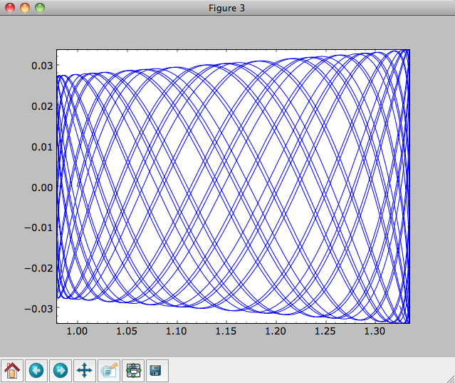
Now we plot the resulting orbit as

>>> o.plot()

Which gives

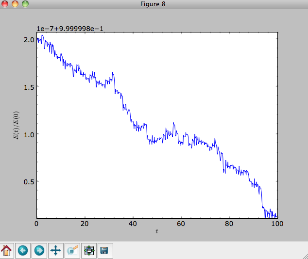
The integrator used is not symplectic, so the energy error grows with time, but is small nonetheless

>>> o.plotE(normed=True)

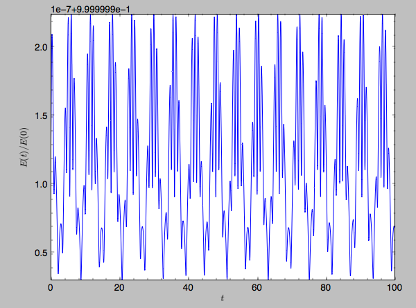
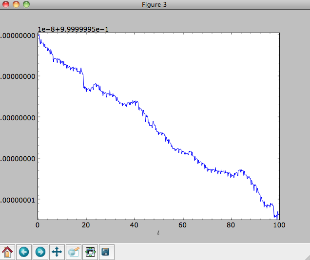
When we use a symplectic leapfrog integrator, we see that the energy error remains constant

>>> o.integrate(ts,mp,method='leapfrog')
>>> o.plotE(xlabel=r'$t$',ylabel=r'$E(t)/E(0)$')

Because stars have typically only orbited the center of their galaxy tens of times, using symplectic integrators is mostly unnecessary (compared to planetary systems which orbits millions or billions of times). galpy contains fast integrators written in C, which can be accessed through the method= keyword (e.g., integrate(...,method='dopr54_c') is a fast high-order Dormand-Prince method).

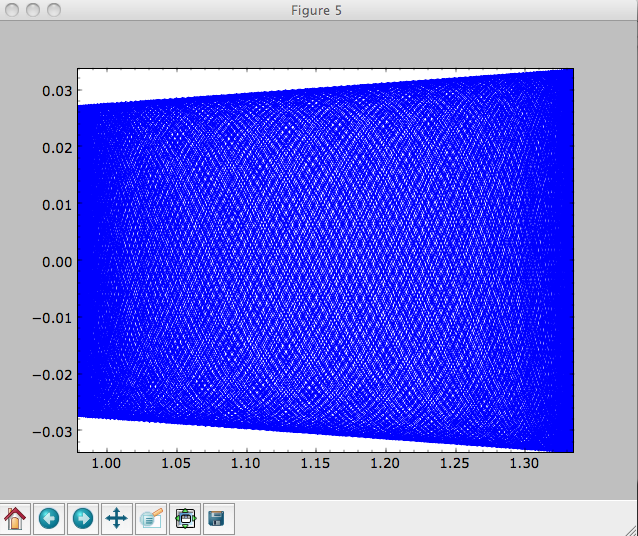
When we integrate for much longer we see how the orbit fills up a torus (this could take a minute)

>>> ts= numpy.linspace(0,1000,10000)
>>> o.integrate(ts,mp,method='odeint')
>>> o.plot()

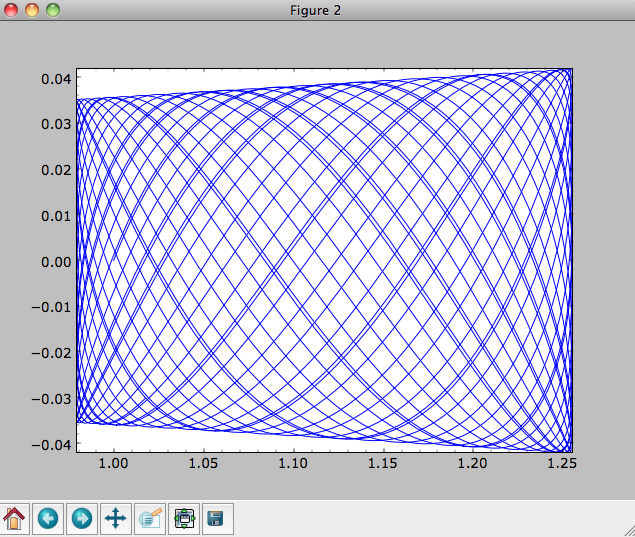
As before, we can also integrate orbits in combinations of potentials. Assuming mp, np, and hp were defined as above, we can

>>> ts= numpy.linspace(0,100,10000)
>>> o.integrate(ts,mp+hp+np)
>>> o.plot()

Energy is again approximately conserved

>>> o.plotE(xlabel=r'$t$',ylabel=r'$E(t)/E(0)$')

Escape velocity curves

Just like we can plot the rotation curve for a potential or a combination of potentials, we can plot the escape velocity curve. For example, the escape velocity curve for the Miyamoto-Nagai disk defined above

>>> mp.plotEscapecurve(Rrange=[0.01,10.],grid=1001)

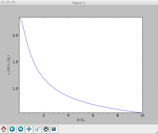
or of the combination of potentials defined above

>>> from galpy.potential import plotEscapecurve
>>> plotEscapecurve(mp+hp+np,Rrange=[0.01,10.],grid=1001)

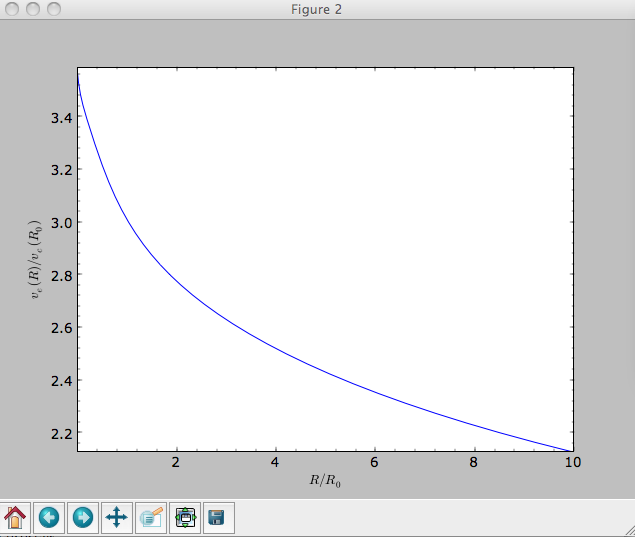
For the Milky-Way-like potential MWPotential2014, the escape-velocity curve is

>>> plotEscapecurve(MWPotential2014,Rrange=[0.01,10.],grid=1001)

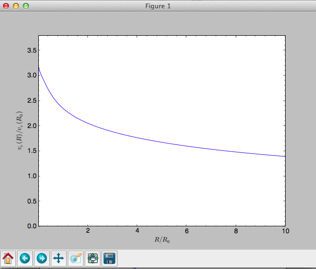
At the solar radius, the escape velocity is

>>> from galpy.potential import vesc
>>> vesc(MWPotential2014,1.)
2.3316389848832784

Or, for a local circular velocity of 220 km/s

>>> vesc(MWPotential2014,1.)*220.
# 512.96057667432126

similar to direct measurements of this (e.g., 2007MNRAS.379..755S and 2014A%26A…562A..91P).