Introduction

The most basic features of galpy are its ability to display rotation curves and perform orbit integration for arbitrary combinations of potentials. This section introduce the most basic features of galpy.potential and galpy.orbit.

Rotation curves

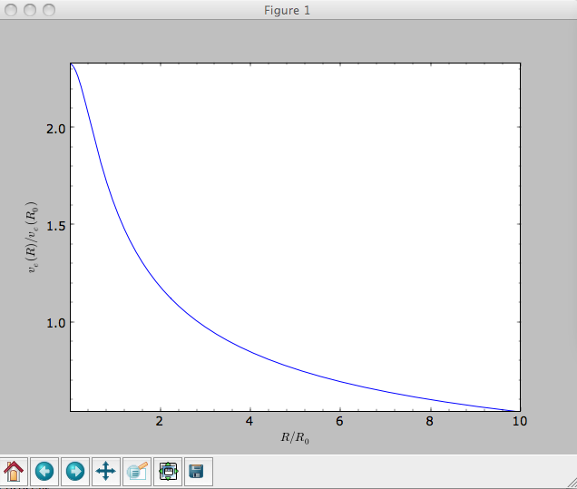
The following code example shows how to initialize a Miyamoto-Nagai disk potential and plot its rotation curve

>>> from galpy.potential import MiyamotoNagaiPotential
>>> mp= MiyamotoNagaiPotential(a=0.5,b=0.0375,normalize=1.)
>>> mp.plotRotcurve(Rrange=[0.01,10.],grid=1001)

The normalize=1. option normalizes the potential such that the radial force is a fraction normalize=1. of the radial force necessary to make the circular velocity 1 at R=1.

Similarly we can initialize other potentials and plot the combined rotation curve

>>> from galpy.potential import NFWPotential, HernquistPotential
>>> mp= MiyamotoNagaiPotential(a=0.5,b=0.0375,normalize=.6)
>>> np= NFWPotential(a=4.5,normalize=.35)
>>> hp= HernquistPotential(a=0.6/8,normalize=0.05)
>>> from galpy.potential import plotRotcurve
>>> plotRotcurve([hp,mp,np],Rrange=[0.01,10.],grid=1001,yrange=[0.,1.2])

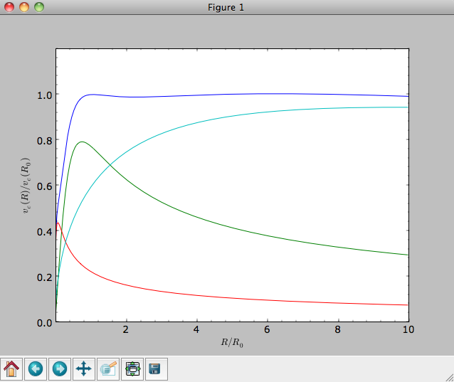
Note that the normalize values add up to 1. such that the circular velocity will be 1 at R=1. The resulting rotation curve is approximately flat. To show the rotation curves of the three components do

>>> mp.plotRotcurve(Rrange=[0.01,10.],grid=1001,overplot=True)
>>> hp.plotRotcurve(Rrange=[0.01,10.],grid=1001,overplot=True)
>>> np.plotRotcurve(Rrange=[0.01,10.],grid=1001,overplot=True)

You’ll see the following

As a shortcut the [hp,mp,np] Milky-Way-like potential is defined as

>>> from galpy.potential import MWPotential

Units in galpy

Above we normalized the potentials such that they give a circular velocity of 1 at R=1. These are the standard galpy units (sometimes referred to as natural units in the documentation). galpy will work most robustly when using these natural units. When using galpy to model a real galaxy with, say, a circular velocity of 220 km/s at R=8 kpc, all of the velocities should be scaled as v= V/[220 km/s] and all of the positions should be scaled as x = X/[8 kpc] when using galpy’s natural units.

For convenience, a utility module bovy_conversion is included in galpy that helps in converting between physical units and natural units for various quantities. For example, in natural units the orbital time of a circular orbit at R=1 is ; in physical units this corresponds to

>>> from galpy.util import bovy_conversion
>>> print 2.*numpy.pi*bovy_conversion.time_in_Gyr(220.,8.)
0.223405444283

or about 223 Myr. We can also express forces in various physical units. For example, for the Milky-Way-like potential defined in galpy, we have that the vertical force at 1.1 kpc is

>>> from galpy.potential import MWPotential, evaluatezforces
>>> -evaluatezforces(1.,1.1/8.,MWPotential)*bovy_conversion.force_in_pcMyr2(220.,8.)
2.3941221528330314

which we can also express as an equivalent surface-density by dividing by

>>> -evaluatezforces(1.,1.1/8.,MWPotential)*bovy_conversion.force_in_2piGmsolpc2(220.,8.)
84.681625645335686

Because the vertical force at the solar circle in the Milky Way at 1.1 kpc above the plane is approximately (e.g., 2013arXiv1309.0809B), this shows that our Milky-Way-like potential has a bit too heavy of a disk.

bovy_conversion further has functions to convert densities, masses, surface densities, and frequencies to physical units (actions are considered to be too obvious to be included); see here for a full list. As a final example, the local dark matter density in the Milky-Way-like potential is given by

>>> MWPotential[1].dens(1.,0.)*bovy_conversion.dens_in_msolpc3(220.,8.)
0.0085853601686596628

or about , in line with current measurements (e.g., 2012ApJ...756...89B).

Orbit integration

We can also integrate orbits in all gaplpy potentials. Going back to a simple Miyamoto-Nagai potential, we initialize an orbit as follows

>>> from galpy.orbit import Orbit
>>> mp= MiyamotoNagaiPotential(a=0.5,b=0.0375,amp=1.,normalize=1.)
>>> o= Orbit(vxvv=[1.,0.1,1.1,0.,0.1])

Since we gave Orbit() a five-dimensional initial condition [R,vR,vT,z,vz], we assume we are dealing with a three-dimensional axisymmetric potential in which we do not wish to track the azimuth. We then integrate the orbit for a set of times ts

>>> import numpy
>>> ts= numpy.linspace(0,100,10000)
>>> o.integrate(ts,mp)

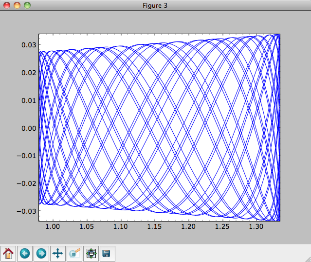
Now we plot the resulting orbit as

>>> o.plot()

Which gives

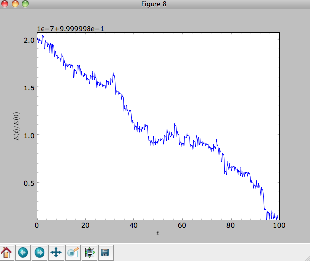
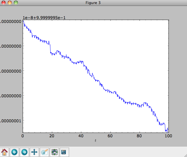
The integrator used is not symplectic, so the energy error grows with time, but is small nonetheless

>>> o.plotE(xlabel=r'$t$',ylabel=r'$E(t)/E(0)$')

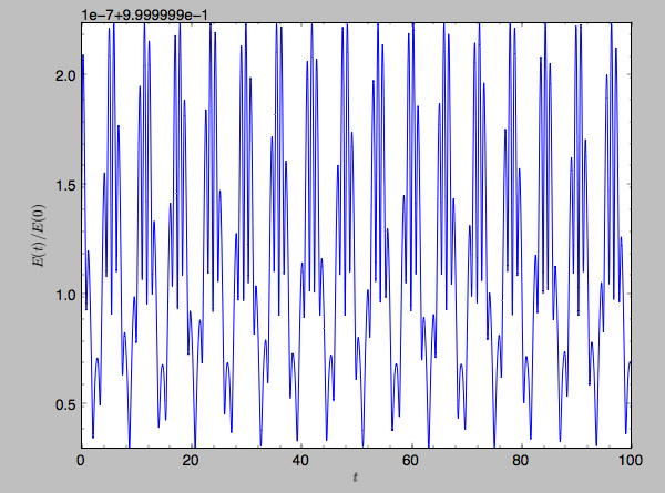
When we use a symplectic leapfrog integrator, we see that the energy error remains constant

>>> o.integrate(ts,mp,method='leapfrog')
>>> o.plotE(xlabel=r'$t$',ylabel=r'$E(t)/E(0)$')

Because stars have typically only orbited the center of their galaxy tens of times, using symplectic integrators is mostly unnecessary (compared to planetary systems which orbits millions or billions of times). galpy contains fast integrators written in C, which can be accessed through the method= keyword (e.g., integrate(...,method='dopr54_c') is a fast high-order Dormand-Prince method).

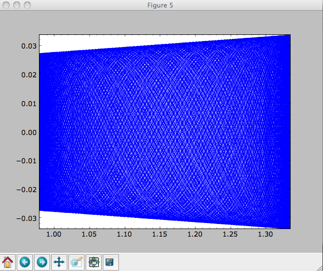
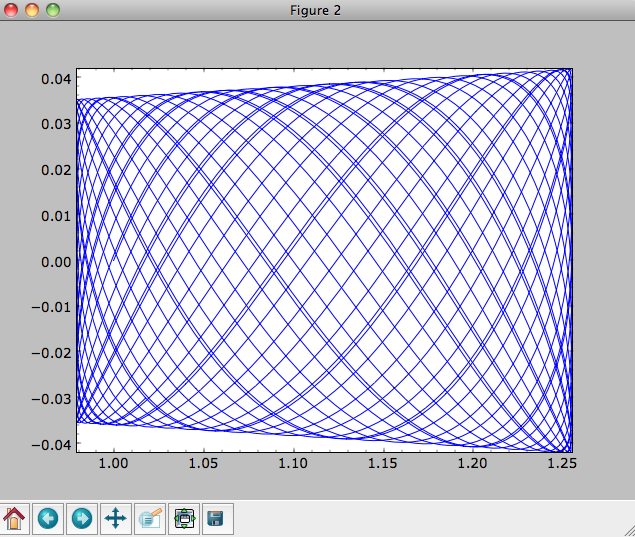
When we integrate for much longer we see how the orbit fills up a torus (this could take a minute)

>>> ts= numpy.linspace(0,1000,10000)
>>> o.integrate(ts,mp)
>>> o.plot()

As before, we can also integrate orbits in combinations of potentials. Assuming mp, np, and hp were defined as above, we can

>>> ts= numpy.linspace(0,100,10000)
>>> o.integrate(ts,[mp,hp,np])
>>> o.plot()

Energy is again approximately conserved

>>> o.plotE(xlabel=r'$t$',ylabel=r'$E(t)/E(0)$')

Escape velocity curves

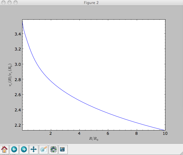
Just like we can plot the rotation curve for a potential or a combination of potentials, we can plot the escape velocity curve. For example, the escape velocity curve for the Miyamoto-Nagai disk defined above

>>> mp.plotEscapecurve(Rrange=[0.01,10.],grid=1001)

or of the combination of potentials defined above

>>> from galpy.potential import plotEscapecurve
>>> plotEscapecurve([mp,hp,np],Rrange=[0.01,10.],grid=1001)