A closer look at orbit integration
Orbit initialization
Standard initialization
Orbits can be initialized in various coordinate frames. The simplest
initialization gives the initial conditions directly in the
Galactocentric cylindrical coordinate frame (or in the rectangular
coordinate frame in one dimension). Orbit() automatically figures
out the dimensionality of the space from the initial conditions in
this case. In three dimensions initial conditions are given either as
vxvv=[R,vR,vT,z,vz,phi] or one can choose not to specify the
azimuth of the orbit and initialize with
vxvv=[R,vR,vT,z,vz]. Since potentials in galpy are easily
initialized to have a circular velocity of one at a radius equal to
one, initial coordinates are best given as a fraction of the radius at
which one specifies the circular velocity, and initial velocities are
best expressed as fractions of this circular velocity. For example,
>>> o= Orbit(vxvv=[1.,0.1,1.1,0.,0.1,0.])
initializes a fully three-dimensional orbit, while
>>> o= Orbit(vxvv=[1.,0.1,1.1,0.,0.1])
initializes an orbit in which the azimuth is not tracked, as might be useful for axisymmetric potentials.
In two dimensions, we can similarly specify fully two-dimensional
orbits o=Orbit(vxvv=[R,vR,vT,phi]) or choose not to track the
azimuth and initialize with o= Orbit(vxvv=[R,vR,vT]).
In one dimension we simply initialize with o= Orbit(vxvv=[x,vx]).
Initialization with physical scales
Orbits are normally used in galpy’s natural coordinates. When Orbits
are initialized using a distance scale ro= and a velocity scale
vo=, then many Orbit methods return quantities in physical
coordinates. Specifically, physical distance and velocity scales are
specified as
>>> op= Orbit(vxvv=[1.,0.1,1.1,0.,0.1,0.],ro=8.,vo=220.)
All output quantities will then be automatically be specified in physical units: kpc for positions, km/s for velocities, (km/s)^2 for energies and the Jacobi integral, km/s kpc for the angular momentum o.L() and actions, 1/Gyr for frequencies, and Gyr for times and periods. See below for examples of this.
Physical units are only used for outputs: internally natural units are
still used and inputs have to also be specified in natural units (for
example, integration times or the time at which an output is requested
must be specified in natural units). If for any output you do not
want the output in physical units, you can specify this by supplying
the keyword argument use_physical=False.
Initialization from observed coordinates
For orbit integration and characterization of observed stars or
clusters, initial conditions can also be specified directly as
observed quantities when radec=True is set. In this case a full
three-dimensional orbit is initialized as o=
Orbit(vxvv=[RA,Dec,distance,pmRA,pmDec,Vlos],radec=True) where RA
and Dec are expressed in degrees, the distance is expressed in kpc,
proper motions are expressed in mas/yr (pmra = pmra’ * cos[Dec] ), and
Vlos is the heliocentric line-of-sight velocity given in
km/s. The observed epoch is currently assumed to be J2000.00. These
observed coordinates are translated to the Galactocentric cylindrical
coordinate frame by assuming a Solar motion that can be specified as
either solarmotion=hogg (default; 2005ApJ…629..268H),
solarmotion=dehnen (1998MNRAS.298..387D) or
solarmotion=shoenrich (2010MNRAS.403.1829S). A circular
velocity can be specified as vo=220 in km/s and a value for the
distance between the Galactic center and the Sun can be given as
ro=8.0 in kpc (e.g., 2012ApJ…759..131B). While the
inputs are given in physical units, the orbit is initialized assuming
a circular velocity of one at the distance of the Sun (that is, the
orbit’s position and velocity is scaled to galpy’s natural units
after converting to the Galactocentric coordinate frame, using the
specified ro= and vo=). The parameters of the coordinate
transformations are stored internally, such that they are
automatically used for relevant outputs (for example, when the RA of
an orbit is requested). An example of all of this is:
>>> o= Orbit(vxvv=[20.,30.,2.,-10.,20.,50.],radec=True,ro=8.,vo=220.)
However, the internally stored position/velocity vector is
>>> print o.vxvv
[1.1476649101960512, 0.20128601278731811, 1.8303776114906387, -0.13107066602923434, 0.58171049004255293, 0.14071341020496472]
and is therefore in natural units.
Similarly, one can also initialize orbits from Galactic coordinates
using o= Orbit(vxvv=[glon,glat,distance,pmll,pmbb,Vlos],lb=True),
where glon and glat are Galactic longitude and latitude expressed in
degrees, and the proper motions are again given in mas/yr ((pmll =
pmll’ * cos[glat] ):
>>> o= Orbit(vxvv=[20.,30.,2.,-10.,20.,50.],lb=True,ro=8.,vo=220.)
>>> print o.vxvv
[0.79998509943955398, 0.075939950035477488, 0.52838231795389867, 0.12812499999999999, 0.89052135379600328, 0.092696334097541536]
When radec=True or lb=True is set, velocities can also be specified in
Galactic coordinates if UVW=True is set. The input is then
vxvv=[RA,Dec,distance,U,V,W], where the velocities are expressed
in km/s. U is, as usual, defined as -vR (minus vR).
When orbits are initialized using radec=True or lb=True,
physical scales ro= and vo= are automatically specified
(because they have defaults of ro=8 and vo=220). Therefore,
all output quantities will be specified in physical units (see
above). If you do want to get outputs in galpy’s natural coordinates,
you can turn this behavior off by doing
>>> o.turn_physical_off()
All outputs will then be specified in galpy’s natural coordinates.
Orbit integration
After an orbit is initialized, we can integrate it for a set of times
ts, given as a numpy array. For example, in a simple logarithmic
potential we can do the following
>>> from galpy.potential import LogarithmicHaloPotential
>>> lp= LogarithmicHaloPotential(normalize=1.)
>>> o= Orbit(vxvv=[1.,0.1,1.1,0.,0.1,0.])
>>> import numpy
>>> ts= numpy.linspace(0,100,10000)
>>> o.integrate(ts,lp)
to integrate the orbit from t=0 to t=100, saving the orbit at
10000 instances.
If we initialize the Orbit using a distance scale ro= and a
velocity scale vo=, then Orbit plots and outputs will use physical
coordinates (currently, times, positions, and velocities)
>>> op= Orbit(vxvv=[1.,0.1,1.1,0.,0.1,0.],ro=8.,vo=220.) #Use Vc=220 km/s at R= 8 kpc as the normalization
>>> op.integrate(ts,lp) #times are still specified in natural coordinates
Displaying the orbit
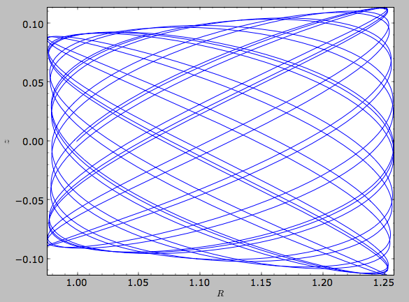
After integrating the orbit, it can be displayed by using the
plot() function. The quantities that are plotted when plot()
is called depend on the dimensionality of the orbit: in 3D the (R,z)
projection of the orbit is shown; in 2D either (X,Y) is plotted if the
azimuth is tracked and (R,vR) is shown otherwise; in 1D (x,vx) is
shown. E.g., for the example given above,
>>> o.plot()
gives
If we do the same for the Orbit that has physical distance and velocity scales associated with it, we get the following
>>> op.plot()
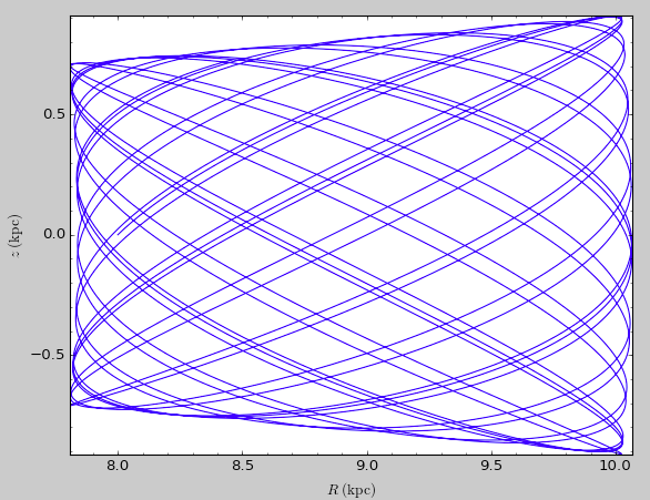
If we call op.plot(use_physical=False), the quantities will be
displayed in natural galpy coordinates.
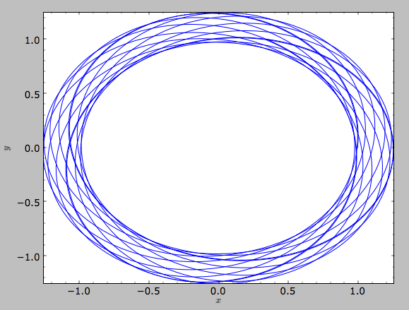
Other projections of the orbit can be displayed by specifying the quantities to plot. E.g.,
>>> o.plot(d1='x',d2='y')
gives the projection onto the plane of the orbit:
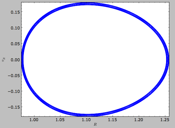
while
>>> o.plot(d1='R',d2='vR')
gives the projection onto (R,vR):
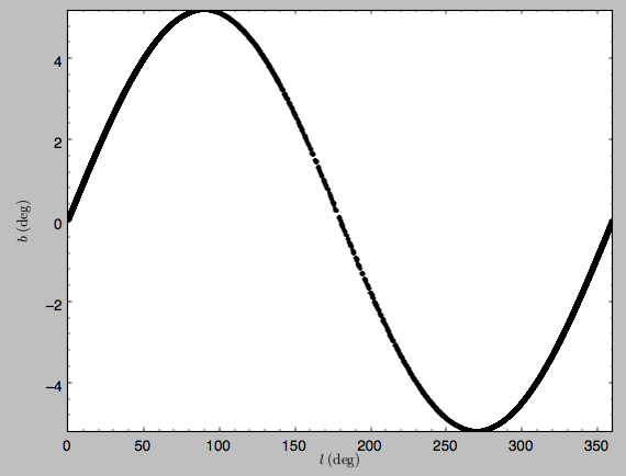
We can also plot the orbit in other coordinate systems such as Galactic longitude and latitude
>>> o.plot('k.',d1='ll',d2='bb')
which shows
or RA and Dec
>>> o.plot('k.',d1='ra',d2='dec')
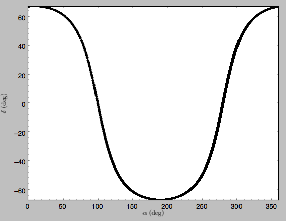
See the documentation of the o.plot function and the o.ra(), o.ll(), etc. functions on how to provide the necessary parameters for the coordinate transformations.
Orbit characterization
The properties of the orbit can also be found using galpy. For example, we can calculate the peri- and apocenter radii of an orbit, its eccentricity, and the maximal height above the plane of the orbit
>>> o.rap(), o.rperi(), o.e(), o.zmax()
(1.2581455175173673,0.97981663263371377,0.12436710999105324,0.11388132751079502)
We can also calculate the energy of the orbit, either in the potential that the orbit was integrated in, or in another potential:
>>> o.E(), o.E(pot=mp)
(0.6150000000000001, -0.67390625000000015)
where mp is the Miyamoto-Nagai potential of Introduction:
Rotation curves.
For the Orbit op that was initialized above with a distance scale
ro= and a velocity scale vo=, these outputs are all in
physical units
>>> op.rap(), op.rperi(), op.e(), op.zmax()
(10.065158988860341,7.8385312810643057,0.12436696983841462,0.91105035688072711) #kpc
>>> op.E(), op.E(pot=mp)
(29766.000000000004, -32617.062500000007) #(km/s)^2
We can also show the energy as a function of time (to check energy conservation)
>>> o.plotE(normed=True)
gives
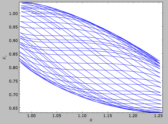
We can specify another quantity to plot the energy against by
specifying d1=. We can also show the vertical energy, for example,
as a function of R
>>> o.plotEz(d1='R',normed=True)
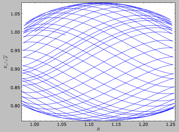
Often, a better approximation to an integral of the motion is given by
Ez/sqrt(density[R]). We refer to this quantity as EzJz and we can plot its
behavior
>>> o.plotEzJz(d1='R',normed=True)
Accessing the raw orbit
The value of R, vR, vT, z, vz, x, vx,
y, vy, phi, and vphi at any time can be obtained by
calling the corresponding function with as argument the time (the same
holds for other coordinates ra, dec, pmra, pmdec,
vra, vdec, ll, bb, pmll, pmbb, vll,
vbb, vlos, dist, helioX, helioY, helioZ,
U, V, and W). If no time is given the initial condition is
returned, and if a time is requested at which the orbit was not saved
spline interpolation is used to return the value. Examples include
>>> o.R(1.)
1.1545076874679474
>>> o.phi(99.)
88.105603035901169
>>> o.ra(2.,obs=[8.,0.,0.],ro=8.)
array([ 285.76403985])
>>> o.helioX(5.)
array([ 1.24888927])
>>> o.pmll(10.,obs=[8.,0.,0.,0.,245.,0.],ro=8.,vo=230.)
array([-6.45263888])
For the Orbit op that was initialized above with a distance scale
ro= and a velocity scale vo=, the first of these would be
>>> op.R(1.)
9.2360614837829225 #kpc
which we can also access in natural coordinates as
>>> op.R(1.,use_physical=False)
1.1545076854728653
We can also specify a different distance or velocity scale on the fly, e.g.,
>>> op.R(1.,ro=4.) #different velocity scale would be vo=
4.6180307418914612
We can also initialize an Orbit instance using the phase-space
position of another Orbit instance evaulated at time t. For
example,
>>> newOrbit= o(10.)
will initialize a new Orbit instance with as initial condition the phase-space position of orbit o at time=10..
The whole orbit can also be obtained using the function getOrbit
>>> o.getOrbit()
which returns a matrix of phase-space points with dimensions [ntimes,ndim].
Fast orbit integration
The standard orbit integration is done purely in python using standard
scipy integrators. When fast orbit integration is needed for batch
integration of a large number of orbits, a set of orbit integration
routines are written in C that can be accessed for most potentials, as
long as they have C implementations, which can be checked by using the
attribute hasC
>>> mp= MiyamotoNagaiPotential(a=0.5,b=0.0375,amp=1.,normalize=1.)
>>> mp.hasC
True
Fast C integrators can be accessed through the method= keyword of
the orbit.integrate method. Currently available integrators are
- rk4_c
- rk6_c
- dopr54_c
which are Runge-Kutta and Dormand-Prince methods. There are also a number of symplectic integrators available
- leapfrog_c
- symplec4_c
- symplec6_c
The higher order symplectic integrators are described in Yoshida (1993).
For most applications I recommend dopr54_c. For example, compare
>>> o= Orbit(vxvv=[1.,0.1,1.1,0.,0.1])
>>> timeit(o.integrate(ts,mp))
1 loops, best of 3: 553 ms per loop
>>> timeit(o.integrate(ts,mp,method='dopr54_c'))
galpyWarning: Using C implementation to integrate orbits
10 loops, best of 3: 25.6 ms per loop
As this example shows, galpy will issue a warning that C is being used. Speed-ups by a factor of 20 are typical.
Integration of the phase-space volume
galpy further supports the integration of the phase-space volume
through the method integrate_dxdv, although this is currently only
implemented for two-dimensional orbits (planarOrbit). As an
example, we can check Liouville’s theorem explicitly. We initialize
the orbit
>>> o= Orbit(vxvv=[1.,0.1,1.1,0.])
and then integrate small deviations in each of the four phase-space directions
>>> ts= numpy.linspace(0.,28.,1001) #~1 Gyr at the Solar circle
>>> o.integrate_dxdv([1.,0.,0.,0.],ts,mp,method='dopr54_c',rectIn=True,rectOut=True)
>>> dx= o.getOrbit_dxdv()[-1,:] # evolution of dxdv[0] along the orbit
>>> o.integrate_dxdv([0.,1.,0.,0.],ts,mp,method='dopr54_c',rectIn=True,rectOut=True)
>>> dy= o.getOrbit_dxdv()[-1,:]
>>> o.integrate_dxdv([0.,0.,1.,0.],ts,mp,method='dopr54_c',rectIn=True,rectOut=True)
>>> dvx= o.getOrbit_dxdv()[-1,:]
>>> o.integrate_dxdv([0.,0.,0.,1.],ts,mp,method='dopr54_c',rectIn=True,rectOut=True)
>>> dvy= o.getOrbit_dxdv()[-1,:]
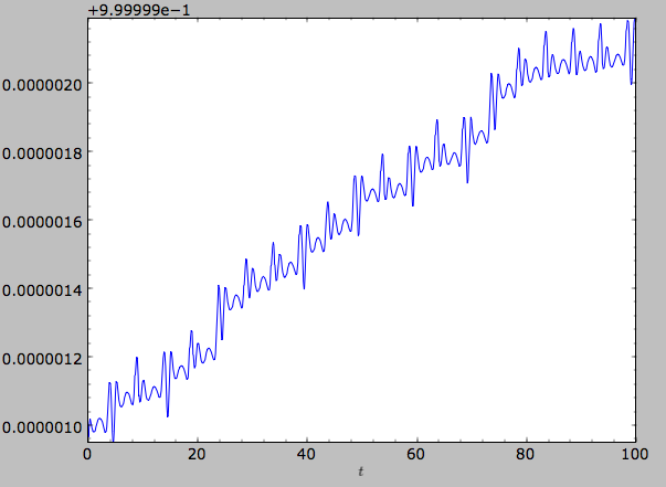
We can then compute the determinant of the Jacobian of the mapping defined by the orbit integration from time zero to the final time
>>> tjac= numpy.linalg.det(numpy.array([dx,dy,dvx,dvy]))
This determinant should be equal to one
>>> print tjac
0.999999991189
>>> numpy.fabs(tjac-1.) < 10.**-8.
True
The calls to integrate_dxdv above set the keywords rectIn= and
rectOut= to True, as the default input and output uses phase-space
volumes defined as (dR,dvR,dvT,dphi) in cylindrical coordinates. When
rectIn or rectOut is set, the in- or output is in rectangular
coordinates ([x,y,vx,vy] in two dimensions).
Implementing the phase-space integration for three-dimensional
FullOrbit instances is straightforward and is part of the longer
term development plan for galpy. Let the main developer know if
you would like this functionality, or better yet, implement it
yourself in a fork of the code and send a pull request!
Example: The eccentricity distribution of the Milky Way’s thick disk
A straightforward application of galpy’s orbit initialization and integration capabilities is to derive the eccentricity distribution of a set of thick disk stars. We start by downloading the sample of SDSS SEGUE (2009AJ….137.4377Y) thick disk stars compiled by Dierickx et al. (2010arXiv1009.1616D) at
http://www.mpia-hd.mpg.de/homes/rix/Data/Dierickx-etal-tab2.txt
After reading in the data (RA,Dec,distance,pmRA,pmDec,vlos; see above)
as a vector vxvv with dimensions [6,ndata] we (a) define the
potential in which we want to integrate the orbits, and (b) integrate
each orbit and save its eccentricity (running this for all 30,000-ish
stars will take about half an hour)
>>> lp= LogarithmicHaloPotential(normalize=1.)
>>> ts= nu.linspace(0.,20.,10000)
>>> mye= nu.zeros(ndata)
>>> for ii in range(len(e)):
...         o= Orbit(vxvv[ii,:],radec=True,vo=220.,ro=8.) #Initialize
...         o.integrate(ts,lp) #Integrate
...         mye[ii]= o.e() #Calculate eccentricity
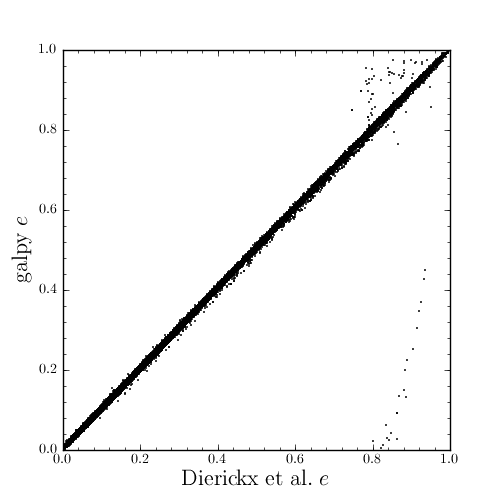
We then find the following eccentricity distribution
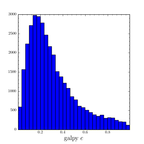
The eccentricity calculated by galpy compare well with those calculated by Dierickx et al., except for a few objects
The script that calculates and plots everything can be downloaded
here.