Potentials in galpy

galpy contains a large variety of potentials in galpy.potential that can be used for orbit integration, the calculation of action-angle coordinates, as part of steady-state distribution functions, and to study the properties of gravitational potentials. This section introduces some of these features.

Potentials and forces

Various 3D and 2D potentials are contained in galpy, list in the API page. Another way to list the latest overview of potentials included with galpy is to run

>>> import galpy.potential
>>> print [p for p in dir(galpy.potential) if 'Potential' in p]
['CosmphiDiskPotential',
 'DehnenBarPotential',
 'DoubleExponentialDiskPotential',
 'EllipticalDiskPotential',
 'FlattenedPowerPotential',
 'HernquistPotential',
....]

(list cut here for brevity). Section Rotation curves explains how to initialize potentials and how to display the rotation curve of single Potential instances or of combinations of such instances. Similarly, we can evaluate a Potential instance

>>> from galpy.potential import MiyamotoNagaiPotential
>>> mp= MiyamotoNagaiPotential(a=0.5,b=0.0375,normalize=1.)
>>> mp(1.,0.)
-1.2889062500000001

Most member functions of Potential instances have corresponding functions in the galpy.potential module that allow them to be evaluated for lists of multiple Potential instances. galpy.potential.MWPotential2014 is such a list of three Potential instances

>>> from galpy.potential import MWPotential2014
>>> print MWPotential2014
[<galpy.potential_src.PowerSphericalPotentialwCutoff.PowerSphericalPotentialwCutoff instance at 0x1089b23b0>, <galpy.potential_src.MiyamotoNagaiPotential.MiyamotoNagaiPotential instance at 0x1089b2320>, <galpy.potential_src.TwoPowerSphericalPotential.NFWPotential instance at 0x1089b2248>]

and we can evaluate the potential by using the evaluatePotentials function

>>> from galpy.potential import evaluatePotentials
>>> evaluatePotentials(1.,0.,MWPotential2014)
-1.3733506513947895

Tip

As discussed in the section on physical units, potentials can be initialized and evaluated with arguments specified as a astropy Quantity with units. Use the configuration parameter apy-units = True to get output values as a Quantity. See also the subsection on Initializing potentials with parameters with units below.

We can plot the potential of axisymmetric potentials (or of non-axisymmetric potentials at phi=0) using the plot member function

>>> mp.plot()

which produces the following plot

Similarly, we can plot combinations of Potentials using plotPotentials, e.g.,

>>> from galpy.potential import plotPotentials
>>> plotPotentials(MWPotential2014,rmin=0.01)

These functions have arguments that can provide custom R and z ranges for the plot, the number of grid points, the number of contours, and many other parameters determining the appearance of these figures.

galpy also allows the forces corresponding to a gravitational potential to be calculated. Again for the Miyamoto-Nagai Potential instance from above

>>> mp.Rforce(1.,0.)
-1.0

This value of -1.0 is due to the normalization of the potential such that the circular velocity is 1. at R=1. Similarly, the vertical force is zero in the mid-plane

>>> mp.zforce(1.,0.)
-0.0

but not further from the mid-plane

>>> mp.zforce(1.,0.125)
-0.53488743705310848

As explained in Units in galpy, these forces are in standard galpy units, and we can convert them to physical units using methods in the galpy.util.bovy_conversion module. For example, assuming a physical circular velocity of 220 km/s at R=8 kpc

>>> from galpy.util import bovy_conversion
>>> mp.zforce(1.,0.125)*bovy_conversion.force_in_kmsMyr(220.,8.)
-3.3095671288657584 #km/s/Myr
>>> mp.zforce(1.,0.125)*bovy_conversion.force_in_2piGmsolpc2(220.,8.)
-119.72021771473301 #2 \pi G Msol / pc^2

Again, there are functions in galpy.potential that allow for the evaluation of the forces for lists of Potential instances, such that

>>> from galpy.potential import evaluateRforces
>>> evaluateRforces(1.,0.,MWPotential2014)
-1.0
>>> from galpy.potential import evaluatezforces
>>> evaluatezforces(1.,0.125,MWPotential2014)*bovy_conversion.force_in_2piGmsolpc2(220.,8.)
>>> -69.680720137571114 #2 \pi G Msol / pc^2

We can evaluate the flattening of the potential as \(\sqrt{|z\,F_R/R\,F_Z|}\) for a Potential instance as well as for a list of such instances

>>> mp.flattening(1.,0.125)
0.4549542914935209
>>> from galpy.potential import flattening
>>> flattening(MWPotential2014,1.,0.125)
0.61231675305658628

Densities

galpy can also calculate the densities corresponding to gravitational potentials. For many potentials, the densities are explicitly implemented, but if they are not, the density is calculated using the Poisson equation (second derivatives of the potential have to be implemented for this). For example, for the Miyamoto-Nagai potential, the density is explicitly implemented

>>> mp.dens(1.,0.)
1.1145444383277576

and we can also calculate this using the Poisson equation

>>> mp.dens(1.,0.,forcepoisson=True)
1.1145444383277574

which are the same to machine precision

>>> mp.dens(1.,0.,forcepoisson=True)-mp.dens(1.,0.)
-2.2204460492503131e-16

Similarly, all of the potentials in galpy.potential.MWPotential2014 have explicitly-implemented densities, so we can do

>>> from galpy.potential import evaluateDensities
>>> evaluateDensities(1.,0.,MWPotential2014)
0.57508603122264867

In physical coordinates, this becomes

>>> evaluateDensities(1.,0.,MWPotential2014)*bovy_conversion.dens_in_msolpc3(220.,8.)
0.1010945632524705 #Msol / pc^3

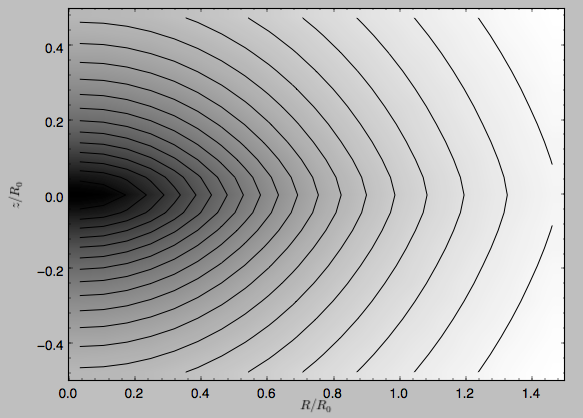
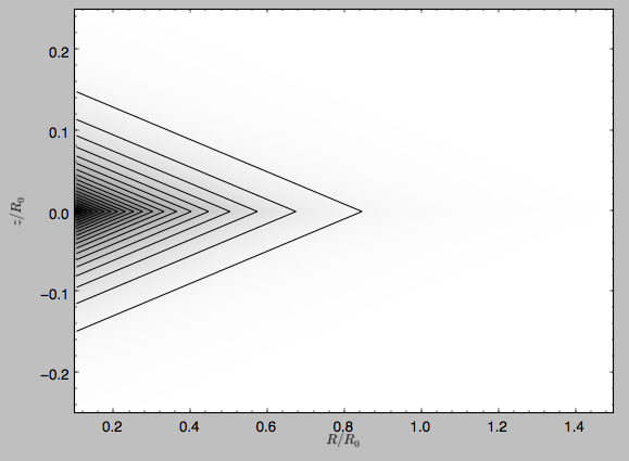
We can also plot densities

>>> from galpy.potential import plotDensities
>>> plotDensities(MWPotential2014,rmin=0.1,zmax=0.25,zmin=-0.25,nrs=101,nzs=101)

which gives

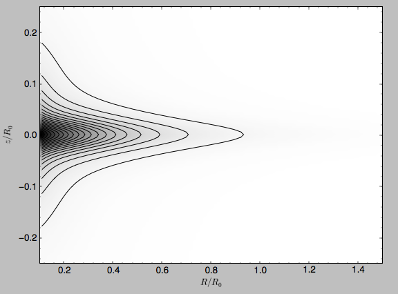
Another example of this is for an exponential disk potential

>>> from galpy.potential import DoubleExponentialDiskPotential
>>> dp= DoubleExponentialDiskPotential(hr=1./4.,hz=1./20.,normalize=1.)

The density computed using the Poisson equation now requires multiple numerical integrations, so the agreement between the analytical density and that computed using the Poisson equation is slightly less good, but still better than a percent

>>> (dp.dens(1.,0.,forcepoisson=True)-dp.dens(1.,0.))/dp.dens(1.,0.)
0.0032522956769123019

The density is

>>> dp.plotDensity(rmin=0.1,zmax=0.25,zmin=-0.25,nrs=101,nzs=101)

and the potential is

>>> dp.plot(rmin=0.1,zmin=-0.25,zmax=0.25)

Clearly, the potential is much less flattened than the density.

Close-to-circular orbits and orbital frequencies

We can also compute the properties of close-to-circular orbits. First of all, we can calculate the circular velocity and its derivative

>>> mp.vcirc(1.)
1.0
>>> mp.dvcircdR(1.)
-0.163777427566978

or, for lists of Potential instances

>>> from galpy.potential import vcirc
>>> vcirc(MWPotential2014,1.)
1.0
>>> from galpy.potential import dvcircdR
>>> dvcircdR(MWPotential2014,1.)
-0.10091361254334696

We can also calculate the various frequencies for close-to-circular orbits. For example, the rotational frequency

>>> mp.omegac(0.8)
1.2784598203204887
>>> from galpy.potential import omegac
>>> omegac(MWPotential2014,0.8)
1.2733514576122869

and the epicycle frequency

>>> mp.epifreq(0.8)
1.7774973530267848
>>> from galpy.potential import epifreq
>>> epifreq(MWPotential2014,0.8)
1.7452189766287691

as well as the vertical frequency

>>> mp.verticalfreq(1.0)
3.7859388972001828
>>> from galpy.potential import verticalfreq
>>> verticalfreq(MWPotential2014,1.)
2.7255405754769875

For close-to-circular orbits, we can also compute the radii of the Lindblad resonances. For example, for a frequency similar to that of the Milky Way’s bar

>>> mp.lindbladR(5./3.,m='corotation') #args are pattern speed and m of pattern
0.6027911166042229 #~ 5kpc
>>> print mp.lindbladR(5./3.,m=2)
None
>>> mp.lindbladR(5./3.,m=-2)
0.9906190683480501

The None here means that there is no inner Lindblad resonance, the m=-2 resonance is in the Solar neighborhood (see the section on the Hercules stream in this documentation).

Using interpolations of potentials

galpy contains a general Potential class interpRZPotential that can be used to generate interpolations of potentials that can be used in their stead to speed up calculations when the calculation of the original potential is computationally expensive (for example, for the DoubleExponentialDiskPotential). Full details on how to set this up are given here. Interpolated potentials can be used anywhere that general three-dimensional galpy potentials can be used. Some care must be taken with outside-the-interpolation-grid evaluations for functions that use C to speed up computations.

NEW in v1.2: Initializing potentials with parameters with units

As already discussed in the section on physical units, potentials in galpy can be specified with parameters with units since v1.2. For most inputs to the initialization it is straightforward to know what type of units the input Quantity needs to have. For example, the scale length parameter a= of a Miyamoto-Nagai disk needs to have units of distance.

The amplitude of a potential is specified through the amp= initialization parameter. The units of this parameter vary from potential to potential. For example, for a logarithmic potential the units are velocity squared, while for a Miyamoto-Nagai potential they are units of mass. Check the documentation of each potential on the API page for the units of the amp= parameter of the potential that you are trying to initialize and please report an Issue if you find any problems with this.

NEW in v1.2: General density/potential pairs with basis-function expansions

galpy allows for the potential and forces of general, time-independent density functions to be computed by expanding the potential and density in terms of basis functions. Currently, only the basis-function expansion of the self-consistent-field (SCF) method of Hernquist & Ostriker (1992) is supported, which works well for ellipsoidal-ish density distributions, but not so well for disk-like density functions.

The basis-function approach in the SCF method is implemented in the SCFPotential class, which is also implemented in C for fast orbit integration. The coefficients of the basis-function expansion can be computed using the scf_compute_coeffs_spherical (for spherically-symmetric density distribution), scf_compute_coeffs_axi (for axisymmetric densities), and scf_compute_coeffs (for the general case). The coefficients obtained from these functions can be directly fed into the SCFPotential initialization. The basis-function expansion has a free scale parameter a, which can be specified for the scf_compute_coeffs_XX functions and for the SCFPotential itself. Make sure that you use the same a! Note that the general functions are quite slow.

The simplest example is that of the Hernquist potential, which is the lowest-order basis function. When we compute the first ten radial coefficients for this density we obtain that only the lowest-order coefficient is non-zero

>>> from galpy.potential import HernquistPotential
>>> from galpy.potential import scf_compute_coeffs_spherical
>>> hp= HernquistPotential(amp=1.,a=2.)
>>> Acos, Asin= scf_compute_coeffs_spherical(hp.dens,10,a=2.)
>>> print(Acos)
array([[[  1.00000000e+00]],
        [[ -2.83370393e-17]],
        [[  3.31150709e-19]],
        [[ -6.66748299e-18]],
        [[  8.19285777e-18]],
        [[ -4.26730651e-19]],
        [[ -7.16849567e-19]],
        [[  1.52355608e-18]],
        [[ -2.24030288e-18]],
        [[ -5.24936820e-19]]])

As a more complicated example, consider a prolate NFW potential

>>> from galpy.potential import TriaxialNFWPotential
>>> np= TriaxialNFWPotential(normalize=1.,c=1.4,a=1.)

and we compute the coefficients using the axisymmetric scf_compute_coeffs_axi

>>> a_SCF= 50. # much larger a than true scale radius works well for NFW
>>> Acos, Asin= scf_compute_coeffs_axi(np.dens,80,40,a=a_SCF)
>>> sp= SCFPotential(Acos=Acos,Asin=Asin,a=a_SCF)

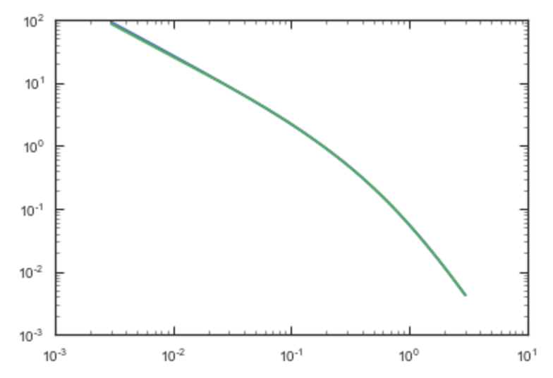
If we compare the densities along the R=Z line as

>>> xs= numpy.linspace(0.,3.,1001)
>>> loglog(xs,np.dens(xs,xs))
>>> loglog(xs,sp.dens(xs,xs))

we get

If we then integrate an orbit, we also get good agreement

>>> from galpy.orbit import Orbit
>>> o= Orbit([1.,0.1,1.1,0.1,0.3,0.])
>>> ts= numpy.linspace(0.,100.,10001)
>>> o.integrate(ts,hp)
>>> o.plotE()
>>> o.integrate(ts,sp)
>>> o.plotE(overplot=True)

which gives

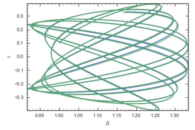
Near the end of the orbit integration, the slight differences between the original potential and the basis-expansion version cause the two orbits to deviate from each other.

The SCFPotential can be used wherever general potentials can be used in galpy.

The potential of N-body simulations

galpy can setup and work with the frozen potential of an N-body simulation. This allows us to study the properties of such potentials in the same way as other potentials in galpy. We can also investigate the properties of orbits in these potentials and calculate action-angle coordinates, using the galpy framework. Currently, this functionality is limited to axisymmetrized versions of the N-body snapshots, although this capability could be somewhat straightforwardly expanded to full triaxial potentials. The use of this functionality requires pynbody to be installed; the potential of any snapshot that can be loaded with pynbody can be used within galpy.

As a first, simple example of this we look at the potential of a single simulation particle, which should correspond to galpy’s KeplerPotential. We can create such a single-particle snapshot using pynbody by doing

>>> import pynbody
>>> s= pynbody.new(star=1)
>>> s['mass']= 1.
>>> s['eps']= 0.

and we get the potential of this snapshot in galpy by doing

>>> from galpy.potential import SnapshotRZPotential
>>> sp= SnapshotRZPotential(s,num_threads=1)

With these definitions, this snapshot potential should be the same as KeplerPotential with an amplitude of one, which we can test as follows

>>> from galpy.potential import KeplerPotential
>>> kp= KeplerPotential(amp=1.)
>>> print(sp(1.1,0.),kp(1.1,0.),sp(1.1,0.)-kp(1.1,0.))
(-0.90909090909090906, -0.9090909090909091, 0.0)
>>> print(sp.Rforce(1.1,0.),kp.Rforce(1.1,0.),sp.Rforce(1.1,0.)-kp.Rforce(1.1,0.))
(-0.82644628099173545, -0.8264462809917353, -1.1102230246251565e-16)

SnapshotRZPotential instances can be used wherever other galpy potentials can be used (note that the second derivatives have not been implemented, such that functions depending on those will not work). For example, we can plot the rotation curve

>>> sp.plotRotcurve()

Because evaluating the potential and forces of a snapshot is computationally expensive, most useful applications of frozen N-body potentials employ interpolated versions of the snapshot potential. These can be setup in galpy using an InterpSnapshotRZPotential class that is a subclass of the interpRZPotential described above and that can be used in the same manner. To illustrate its use we will make use of one of pynbody’s example snapshots, g15784. This snapshot is used here to illustrate pynbody’s use. Please follow the instructions there on how to download this snapshot.

Once you have downloaded the pynbody testdata, we can load this snapshot using

>>> s = pynbody.load('testdata/g15784.lr.01024.gz')

(please adjust the path according to where you downloaded the pynbody testdata). We get the main galaxy in this snapshot, center the simulation on it, and align the galaxy face-on using

>>> h = s.halos()
>>> h1 = h[1]
>>> pynbody.analysis.halo.center(h1,mode='hyb')
>>> pynbody.analysis.angmom.faceon(h1, cen=(0,0,0),mode='ssc')

we also convert the simulation to physical units, but set G=1 by doing the following

>>> s.physical_units()
>>> from galpy.util.bovy_conversion import _G
>>> g= pynbody.array.SimArray(_G/1000.)
>>> g.units= 'kpc Msol**-1 km**2 s**-2 G**-1'
>>> s._arrays['mass']= s._arrays['mass']*g

We can now load an interpolated version of this snapshot’s potential into galpy using

>>> from galpy.potential import InterpSnapshotRZPotential
>>> spi= InterpSnapshotRZPotential(h1,rgrid=(numpy.log(0.01),numpy.log(20.),101),logR=True,zgrid=(0.,10.,101),interpPot=True,zsym=True)

where we further assume that the potential is symmetric around the mid-plane (z=0). This instantiation will take about ten to fiteen minutes. This potential instance has physical units (and thus the rgrid= and zgrid= inputs are given in kpc if the simulation’s distance unit is kpc). For example, if we ask for the rotation curve, we get the following:

>>> spi.plotRotcurve(Rrange=[0.01,19.9],xlabel=r'$R\,(\mathrm{kpc})$',ylabel=r'$v_c(R)\,(\mathrm{km\,s}^{-1})$')

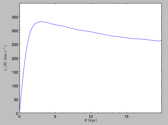
This can be compared to the rotation curve calculated by pynbody, see here.

Because galpy works best in a system of natural units as explained in Units in galpy, we will convert this instance to natural units using the circular velocity at R=10 kpc, which is

>>> spi.vcirc(10.)
294.62723076942245

To convert to natural units we do

>>> spi.normalize(R0=10.)

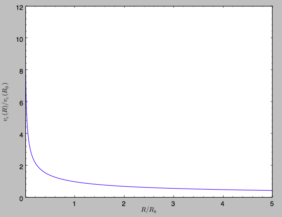
We can then again plot the rotation curve, keeping in mind that the distance unit is now \(R_0\)

>>> spi.plotRotcurve(Rrange=[0.01,1.99])

which gives

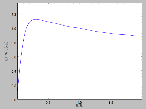
in particular

>>> spi.vcirc(1.)
1.0000000000000002

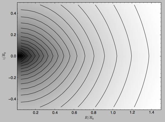
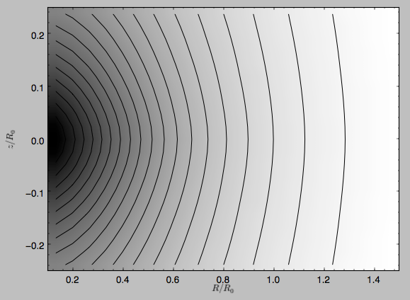
We can also plot the potential

>>> spi.plot(rmin=0.01,rmax=1.9,nrs=51,zmin=-0.99,zmax=0.99,nzs=51)

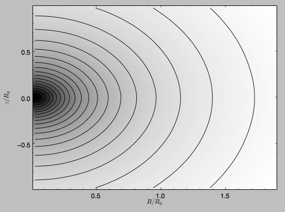
Clearly, this simulation’s potential is quite spherical, which is confirmed by looking at the flattening

>>> spi.flattening(1.,0.1)
0.86675711023391921
>>> spi.flattening(1.5,0.1)
0.94442750306256895

The epicyle and vertical frequencies can also be interpolated by setting the interpepifreq=True or interpverticalfreq=True keywords when instantiating the InterpSnapshotRZPotential object.

Conversion to NEMO potentials

NEMO is a set of tools for studying stellar dynamics. Some of its functionality overlaps with that of galpy, but many of its programs are very complementary to galpy. In particular, it has the ability to perform N-body simulations with a variety of poisson solvers, which is currently not supported by galpy (and likely will never be directly supported). To encourage interaction between galpy and NEMO it is quite useful to be able to convert potentials between these two frameworks, which is not completely trivial. In particular, NEMO contains Walter Dehnen’s fast collisionless gyrfalcON code (see 2000ApJ…536L..39D and 2002JCoPh.179…27D) and the discussion here focuses on how to run N-body simulations using external potentials defined in galpy.

Some galpy potential instances support the functions nemo_accname and nemo_accpars that return the name of the NEMO potential corresponding to this galpy Potential and its parameters in NEMO units. These functions assume that you use NEMO with WD_units, that is, positions are specified in kpc, velocities in kpc/Gyr, times in Gyr, and G=1. For the Miyamoto-Nagai potential above, you can get its name in the NEMO framework as

>>> mp.nemo_accname()
'MiyamotoNagai'

and its parameters as

>>> mp.nemo_accpars(220.,8.)
'0,592617.11132,4.0,0.3'

assuming that we scale velocities by vo=220 km/s and positions by ro=8 kpc in galpy. These two strings can then be given to the gyrfalcON accname= and accpars= keywords.

We can do the same for lists of potentials. For example, for MWPotential2014 we do

>>> from galpy.potential import nemo_accname, nemo_accpars
>>> nemo_accname(MWPotential2014)
'PowSphwCut+MiyamotoNagai+NFW'
>>> nemo_accpars(MWPotential2014,220.,8.)
'0,1001.79126907,1.8,1.9#0,306770.418682,3.0,0.28#0,16.0,162.958241887'

Therefore, these are the accname= and accpars= that one needs to provide to gyrfalcON to run a simulation in MWPotential2014.

Note that the NEMO potential PowSphwCut is not a standard NEMO potential. This potential can be found in the nemo/ directory of the galpy source code; this directory also contains a Makefile that can be used to compile the extra NEMO potential and install it in the correct NEMO directory (this requires one to have NEMO running, i.e., having sourced nemo_start).

You can use the PowSphwCut.cc file in the nemo/ directory as a template for adding additional potentials in galpy to the NEMO framework. To figure out how to convert the normalized galpy potential to an amplitude when scaling to physical coordinates (like kpc and kpc/Gyr), one needs to look at the scaling of the radial force with R. For example, from the definition of MiyamotoNagaiPotential, we see that the radial force scales as \(R^{-2}\). For a general scaling \(R^{-\alpha}\), the amplitude will scale as \(V_0^2\,R_0^{\alpha-1}\) with the velocity \(V_0\) and position \(R_0\) of the v=1 at R=1 normalization. Therefore, for the MiyamotoNagaiPotential, the physical amplitude scales as \(V_0^2\,R_0\). For the LogarithmicHaloPotential, the radial force scales as \(R^{-1}\), so the amplitude scales as \(V_0^2\).

Currently, only the MiyamotoNagaiPotential, NFWPotential, PowerSphericalPotentialwCutoff, PlummerPotential, MN3ExponentialDiskPotential, and the LogarithmicHaloPotential have this NEMO support. Combinations of the first three are also supported (e.g., MWPotential2014); they can also be combined with spherical LogarithmicHaloPotentials. Because of the definition of the logarithmic potential in NEMO, it cannot be flattened in z, so to use a flattened logarithmic potential, one has to flip y and z between galpy and NEMO (one can flatten in y).

Adding potentials to the galpy framework

Potentials in galpy can be used in many places such as orbit integration, distribution functions, or the calculation of action-angle variables, and in most cases any instance of a potential class that inherits from the general Potential class (or a list of such instances) can be given. For example, all orbit integration routines work with any list of instances of the general Potential class. Adding new potentials to galpy therefore allows them to be used everywhere in galpy where general Potential instances can be used. Adding a new class of potentials to galpy consists of the following series of steps (some of these are also given in the file README.dev in the galpy distribution):

1. Implement the new potential in a class that inherits from galpy.potential.Potential. The new class should have an __init__ method that sets up the necessary parameters for the class. An amplitude parameter amp= and two units parameters ro= and vo= should be taken as an argument for this class and before performing any other setup, the galpy.potential.Potential.__init__(self,amp=amp,ro=ro,vo=vo,amp_units=) method should be called to setup the amplitude and the system of units; the amp_units= keyword specifies the physical units of the amplitude parameter (e.g., amp_units='velocity2' when the units of the amplitude are velocity-squared) To add support for normalizing the potential to standard galpy units, one can call the galpy.potential.Potential.normalize function at the end of the __init__ function.

The new potential class should implement some of the following functions:

• _evaluate(self,R,z,phi=0,t=0) which evaluates the potential itself (without the amp factor, which is added in the __call__ method of the general Potential class).
• _Rforce(self,R,z,phi=0.,t=0.) which evaluates the radial force in cylindrical coordinates (-d potential / d R).
• _zforce(self,R,z,phi=0.,t=0.) which evaluates the vertical force in cylindrical coordinates (-d potential / d z).
• _R2deriv(self,R,z,phi=0.,t=0.) which evaluates the second (cylindrical) radial derivative of the potential (d^2 potential / d R^2).
• _z2deriv(self,R,z,phi=0.,t=0.) which evaluates the second (cylindrical) vertical derivative of the potential (d^2 potential / d z^2).
• _Rzderiv(self,R,z,phi=0.,t=0.) which evaluates the mixed (cylindrical) radial and vertical derivative of the potential (d^2 potential / d R d z).
• _dens(self,R,z,phi=0.,t=0.) which evaluates the density. If not given, the density is computed using the Poisson equation from the first and second derivatives of the potential (if all are implemented).
• _mass(self,R,z=0.,t=0.) which evaluates the mass. For spherical potentials this should give the mass enclosed within the spherical radius; for axisymmetric potentials this should return the mass up to R and between -Z and Z. If not given, the mass is computed by integrating the density (if it is implemented or can be calculated from the Poisson equation).
• _phiforce(self,R,z,phi=0.,t=0.): the azimuthal force in cylindrical coordinates (assumed zero if not implemented).
• _phi2deriv(self,R,z,phi=0.,t=0.): the second azimuthal derivative of the potential in cylindrical coordinates (d^2 potential / d phi^2; assumed zero if not given).
• _Rphideriv(self,R,z,phi=0.,t=0.): the mixed radial and azimuthal derivative of the potential in cylindrical coordinates (d^2 potential / d R d phi; assumed zero if not given).

If you want to be able to calculate the concentration for a potential, you also have to set self._scale to a scale parameter for your potential.

The code for galpy.potential.MiyamotoNagaiPotential gives a good template to follow for 3D axisymmetric potentials. Similarly, the code for galpy.potential.CosmphiDiskPotential provides a good template for 2D, non-axisymmetric potentials.

After this step, the new potential will work in any part of galpy that uses pure python potentials. To get the potential to work with the C implementations of orbit integration or action-angle calculations, the potential also has to be implemented in C and the potential has to be passed from python to C.

The __init__ method should be written in such a way that a relevant object can be initialized using Classname() (i.e., there have to be reasonable defaults given for all parameters, including the amplitude); doing this allows the nose tests for potentials to automatically check that your Potential’s potential function, force functions, second derivatives, and density (through the Poisson equation) are correctly implemented (if they are implemented). The continuous-integration platform that builds the galpy codebase upon code pushes will then automatically test all of this, streamlining push requests of new potentials.

2. To add a C implementation of the potential, implement it in a .c file under potential_src/potential_c_ext. Look at potential_src/potential_c_ext/LogarithmicHaloPotential.c for the right format for 3D, axisymmetric potentials, or at potential_src/potential_c_ext/LopsidedDiskPotential.c for 2D, non-axisymmetric potentials.

For orbit integration, the functions such as:

• double LogarithmicHaloPotentialRforce(double R,double Z, double phi,double t,struct potentialArg * potentialArgs)
• double LogarithmicHaloPotentialzforce(double R,double Z, double phi,double t,struct potentialArg * potentialArgs)

are most important. For some of the action-angle calculations

• double LogarithmicHaloPotentialEval(double R,double Z, double phi,double t,struct potentialArg * potentialArgs)

is most important (i.e., for those algorithms that evaluate the potential). The arguments of the potential are passed in a potentialArgs structure that contains args, which are the arguments that should be unpacked. Again, looking at some example code will make this clear. The potentialArgs structure is defined in potential_src/potential_c_ext/galpy_potentials.h.

3. Add the potential’s function declarations to potential_src/potential_c_ext/galpy_potentials.h

4. (4. and 5. for planar orbit integration) Edit the code under orbit_src/orbit_c_ext/integratePlanarOrbit.c to set up your new potential (in the parse_leapFuncArgs function).

5. Edit the code in orbit_src/integratePlanarOrbit.py to set up your new potential (in the _parse_pot function).

6. Edit the code under orbit_src/orbit_c_ext/integrateFullOrbit.c to set up your new potential (in the parse_leapFuncArgs_Full function).

7. Edit the code in orbit_src/integrateFullOrbit.py to set up your new potential (in the _parse_pot function).

8. (for using the actionAngleStaeckel methods in C) Edit the code in actionAngle_src/actionAngle_c_ext/actionAngle.c to parse the new potential (in the parse_actionAngleArgs function).

9. Finally, add self.hasC= True to the initialization of the potential in question (after the initialization of the super class, or otherwise it will be undone). If you have implemented the necessary second derivatives for integrating phase-space volumes, also add self.hasC_dxdv=True.

After following the relevant steps, the new potential class can be used in any galpy context in which C is used to speed up computations.