This page was generated from a Jupyter notebook. You can download it here.

Action-Angle Coordinates: Adiabatic Approximation

The adiabatic approximation (actionAngleAdiabatic) separates the radial and vertical motions, computing \(J_z\) at each radius while assuming that the radial motion is slow compared to the vertical oscillation (e.g., Binney & McMillan 2010). This is fast but less accurate than the Staeckel method for orbits with large vertical excursions.

Warning

Frequencies and angles using the adiabatic approximation are not implemented at this time. Use the Staeckel approximation if you need frequencies and angles.

%matplotlib inline
import numpy
import matplotlib.pyplot as plt
from galpy.potential import MWPotential2014
from galpy.orbit import Orbit
import warnings

warnings.filterwarnings("ignore", category=RuntimeWarning)
warnings.filterwarnings("ignore", category=UserWarning)

Setup

Setup is straightforward. Using c=True gives a significant speed-up (about 50x for single evaluations, 200x for arrays):

from galpy.actionAngle import actionAngleAdiabatic

aAA = actionAngleAdiabatic(pot=MWPotential2014, c=True)

Computing actions

Calling the object returns \((J_R, L_z, J_z)\):

jr_ad, jphi_ad, jz_ad = aAA(1.0, 0.1, 1.1, 0.0, 0.05)
print(f"J_R = {jr_ad.item():.6f}, L_z = {jphi_ad.item():.6f}, J_z = {jz_ad.item():.6f}")

J_R = 0.013525, L_z = 1.100000, J_z = 0.000469

Action conservation for a thin-disk orbit

The adiabatic approximation works well for orbits that stay close to the plane. Let’s check action conservation for a near-circular orbit:

o = Orbit([1.0, 0.1, 1.1, 0.0, 0.05])
ts = numpy.linspace(0, 100, 1001)
o.integrate(ts, MWPotential2014)

print(f"Maximum height: {o.zmax() * 8.0:.2f} kpc (for R_0 = 8 kpc)")

Maximum height: 0.18 kpc (for R_0 = 8 kpc)

Now compute the actions along the orbit and check conservation:

js = aAA(o.R(ts), o.vR(ts), o.vT(ts), o.z(ts), o.vz(ts))

plt.plot(ts, numpy.log10(numpy.fabs((js[0] - numpy.mean(js[0])) / numpy.mean(js[0]))))
plt.plot(ts, numpy.log10(numpy.fabs((js[2] - numpy.mean(js[2])) / numpy.mean(js[2]))))
plt.xlabel(r"$t$")
plt.ylabel(r"$\log_{10}|\Delta J / \langle J \rangle|$")
plt.legend([r"$J_R$", r"$J_z$"])
plt.title("Adiabatic: action conservation (thin-disk orbit)");

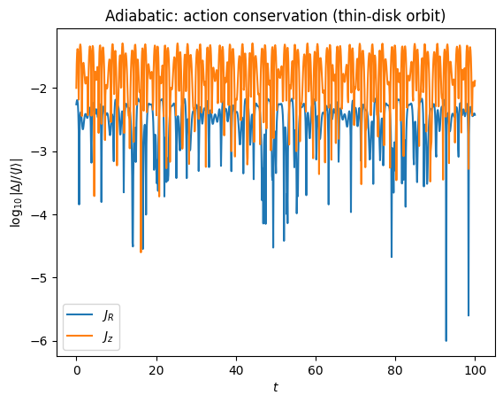
The radial action is conserved to about half a percent, the vertical action to about two percent.

Comparison with Staeckel for thin-disk orbits

For thin-disk orbits, the adiabatic and Staeckel approximations agree well:

from galpy.actionAngle import actionAngleStaeckel

aAS = actionAngleStaeckel(pot=MWPotential2014, delta=0.4, c=True)

jr_st, jphi_st, jz_st = aAS(1.0, 0.1, 1.1, 0.0, 0.05)

print("Method       J_R        J_z")
print(f"Adiabatic:   {jr_ad.item():.6f}   {jz_ad.item():.6f}")
print(f"Staeckel:    {jr_st.item():.6f}   {jz_st.item():.6f}")
print(
    f"Difference:   {jr_st.item() - jr_ad.item():.6f}   {jz_st.item() - jz_ad.item():.6f}"
)

Method       J_R        J_z
Adiabatic:   0.013525   0.000469
Staeckel:    0.013636   0.000463
Difference:   0.000111   -0.000006

Failure for high-z orbits

The adiabatic approximation breaks down for orbits that reach distances of a kpc and more from the plane. Let’s examine a higher-z orbit:

o_hz = Orbit([1.0, 0.1, 1.1, 0.0, 0.25])
o_hz.integrate(ts, MWPotential2014)

print(f"Maximum height: {o_hz.zmax() * 8.0:.2f} kpc (for R_0 = 8 kpc)")

Maximum height: 1.35 kpc (for R_0 = 8 kpc)

Compute actions along this higher-z orbit:

js_hz = aAA(o_hz.R(ts), o_hz.vR(ts), o_hz.vT(ts), o_hz.z(ts), o_hz.vz(ts))

plt.plot(
    ts,
    numpy.log10(numpy.fabs((js_hz[0] - numpy.mean(js_hz[0])) / numpy.mean(js_hz[0]))),
)
plt.plot(
    ts,
    numpy.log10(numpy.fabs((js_hz[2] - numpy.mean(js_hz[2])) / numpy.mean(js_hz[2]))),
)
plt.xlabel(r"$t$")
plt.ylabel(r"$\log_{10}|\Delta J / \langle J \rangle|$")
plt.legend([r"$J_R$", r"$J_z$"])
plt.title("Adiabatic: action conservation (high-z orbit)");

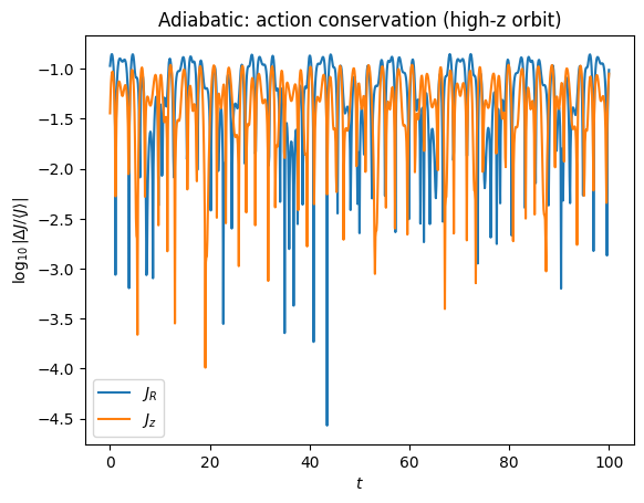
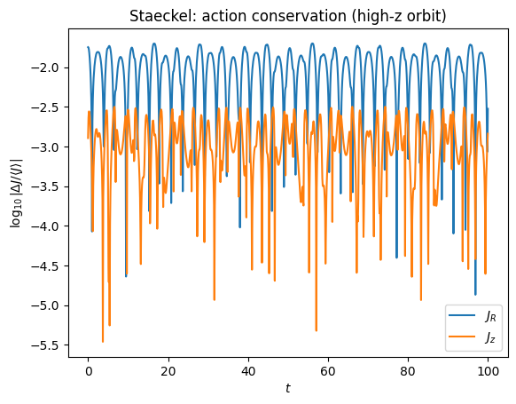
The radial action is now only conserved to about ten percent and the vertical action to approximately five percent. The Staeckel approximation does much better for the same orbit (better than a percent for \(J_R\) and a fraction of a percent for \(J_z\)):

jr_st, jphi_st, jz_st = aAS(
    o_hz.R(ts), o_hz.vR(ts), o_hz.vT(ts), o_hz.z(ts), o_hz.vz(ts)
)

plt.plot(ts, numpy.log10(numpy.fabs((jr_st - numpy.mean(jr_st)) / numpy.mean(jr_st))))
plt.plot(ts, numpy.log10(numpy.fabs((jz_st - numpy.mean(jz_st)) / numpy.mean(jz_st))))
plt.xlabel(r"$t$")
plt.ylabel(r"$\log_{10}|\Delta J / \langle J \rangle|$")
plt.legend([r"$J_R$", r"$J_z$"])
plt.title("Staeckel: action conservation (high-z orbit)");

Grid-based interpolation: actionAngleAdiabaticGrid

Like the Staeckel method, the adiabatic approximation can be sped up with a precomputed grid. The grid-based calculation can be significantly faster than even the direct C implementation (up to 150x for large arrays):

from galpy.actionAngle import actionAngleAdiabaticGrid

aAAG = actionAngleAdiabaticGrid(
    pot=MWPotential2014, c=True, nR=31, nEz=31, nEr=51, nLz=51
)

Compare the grid-based and direct calculations:

jr_direct, _, jz_direct = aAA(1.0, 0.1, 1.1, 0.0, 0.05)
jr_grid, _, jz_grid = aAAG(1.0, 0.1, 1.1, 0.0, 0.05)

print(
    f"J_R: direct = {jr_direct.item():.6f}, grid = {jr_grid.item():.6f}, difference = {jr_grid.item() - jr_direct.item():.6f}"
)
print(
    f"J_z: direct = {jz_direct.item():.6f}, grid = {jz_grid.item():.6f}, difference = {jz_grid.item() - jz_direct.item():.6f}"
)

J_R: direct = 0.013525, grid = 0.013527, difference = 0.000002
J_z: direct = 0.000469, grid = 0.000477, difference = 0.000008

The grid-based and direct calculations agree well. For MWPotential2014 and other more complicated potentials (such as those involving a double-exponential disk), the overhead of setting up the grid is worth it when evaluating more than a few thousand actions.

Using the Orbit interface

Actions and orbital parameters can also be computed directly from Orbit objects using o.jr(), o.jz(), o.e(analytic=True, type='adiabatic'), etc. The Orbit interface auto-determines the action-angle method and delta parameter. For the adiabatic approximation, specify type='adiabatic' when computing orbital parameters analytically:

# Using the Orbit interface for the adiabatic approximation
o_orb = Orbit([1.0, 0.1, 1.1, 0.0, 0.05])

# Orbital parameters with the adiabatic approximation (no integration needed)
print(
    "Eccentricity (adiabatic):",
    o_orb.e(analytic=True, pot=MWPotential2014, type="adiabatic"),
)
print(
    "Apocenter (adiabatic):",
    o_orb.rap(analytic=True, pot=MWPotential2014, type="adiabatic"),
)
print(
    "zmax (adiabatic):",
    o_orb.zmax(analytic=True, pot=MWPotential2014, type="adiabatic"),
)

# Compare with Staeckel (generally more accurate)
print(
    "\nEccentricity (staeckel):",
    o_orb.e(analytic=True, pot=MWPotential2014, type="staeckel"),
)
print(
    "Apocenter (staeckel):",
    o_orb.rap(analytic=True, pot=MWPotential2014, type="staeckel"),
)
print(
    "zmax (staeckel):", o_orb.zmax(analytic=True, pot=MWPotential2014, type="staeckel")
)

Eccentricity (adiabatic): 0.13474166226188383
Apocenter (adiabatic): 1.2838439076540742
zmax (adiabatic): 0.018896497628549124

Eccentricity (staeckel): 0.13508986478572993
Apocenter (staeckel): 1.2848214705139953
zmax (staeckel): 0.022401525812555927