This page was generated from a Jupyter notebook. You can download it here.

Action-Angle Coordinates: Staeckel Approximation

The Staeckel approximation (actionAngleStaeckel) is the most accurate general method for computing actions in axisymmetric potentials. It works by locally approximating the potential as a Staeckel potential (separable in confocal ellipsoidal coordinates), following the algorithm of Binney (2012).

For all intents and purposes, the Staeckel approximation makes the adiabatic approximation obsolete: it is as fast and more precise. The only additional requirement is that the user must specify a focal length \(\Delta\), but this can be easily estimated from the potential.

For an introduction to action-angle coordinates and simpler methods, see the Introduction. For the orbit-integration-based method that works for highly eccentric orbits, see IsochroneApprox.

%matplotlib inline
import numpy
import matplotlib.pyplot as plt
from galpy.potential import MWPotential2014
from galpy.orbit import Orbit
import warnings

warnings.filterwarnings("ignore", category=RuntimeWarning)
warnings.filterwarnings("ignore", category=UserWarning)

Setup

The key parameter is delta, the focus of the confocal coordinate system. You can estimate an appropriate value using estimateDeltaStaeckel, which estimates \(\Delta\) from the second derivatives of the potential (see Sanders 2012):

from galpy.actionAngle import actionAngleStaeckel, estimateDeltaStaeckel

# Estimate delta for an orbit near R=1, z=0
delta = estimateDeltaStaeckel(MWPotential2014, 1.0, 0.0)
print("Estimated delta:", delta)

Estimated delta: 0.7013326670567281

For more accuracy, you can estimate delta along an integrated orbit by averaging (through the median) estimates at positions around the orbit:

o = Orbit([1.0, 0.1, 1.1, 0.0, 0.25, 0.0])
ts = numpy.linspace(0, 100, 1001)
o.integrate(ts, MWPotential2014)

# Estimate delta from the orbit's R and z range
delta_orbit = estimateDeltaStaeckel(MWPotential2014, o.R(ts), o.z(ts))
print("Delta from orbit:", delta_orbit)

Delta from orbit: 0.40272708628053305

We will use \(\Delta = 0.4\) in what follows. We set up the actionAngleStaeckel object with c=True to use the fast C implementation:

aAS = actionAngleStaeckel(pot=MWPotential2014, delta=0.4, c=True)

Computing actions

Calling the object returns \((J_R, L_z, J_z)\):

jr, jphi, jz = aAS(1.0, 0.1, 1.1, 0.0, 0.05)
print(f"J_R = {jr.item():.6f}, L_z = {jphi.item():.6f}, J_z = {jz.item():.6f}")

J_R = 0.013636, L_z = 1.100000, J_z = 0.000463

For the orbit with higher vertical excursion:

jr_hz, jphi_hz, jz_hz = aAS(o.R(), o.vR(), o.vT(), o.z(), o.vz())
print(f"J_R = {jr_hz.item():.6f}, L_z = {jphi_hz.item():.6f}, J_z = {jz_hz.item():.6f}")

J_R = 0.019222, L_z = 1.100000, J_z = 0.015277

Computing actions, frequencies, and angles

The actionsFreqs method returns \((J_R, L_z, J_z, \Omega_R, \Omega_\phi, \Omega_z)\):

jr, jphi, jz, Or, Op, Oz = aAS.actionsFreqs(1.0, 0.1, 1.1, 0.0, 0.05)
print(f"J_R = {jr.item():.6f}, L_z = {jphi.item():.6f}, J_z = {jz.item():.6f}")
print(
    f"Omega_R = {Or.item():.4f}, Omega_phi = {Op.item():.4f}, Omega_z = {Oz.item():.4f}"
)

J_R = 0.013636, L_z = 1.100000, J_z = 0.000463
Omega_R = 1.1595, Omega_phi = 0.8682, Omega_z = 2.1432

The actionsFreqsAngles method additionally returns the angles \((\theta_R, \theta_\phi, \theta_z)\). Note that you must specify phi for the angles:

jr, jphi, jz, Or, Op, Oz, wr, wp, wz = aAS.actionsFreqsAngles(
    1.0, 0.1, 1.1, 0.0, 0.05, 0.0
)
print(f"J_R = {jr.item():.6f}")
print(
    f"Omega_R = {Or.item():.4f}, Omega_phi = {Op.item():.4f}, Omega_z = {Oz.item():.4f}"
)
print(
    f"theta_R = {wr.item():.4f}, theta_phi = {wp.item():.4f}, theta_z = {wz.item():.4f}"
)

J_R = 0.013636
Omega_R = 1.1595, Omega_phi = 0.8682, Omega_z = 2.1432
theta_R = 0.4687, theta_phi = 6.1767, theta_z = 6.0535

Warning

Frequencies and angles using the Staeckel approximation are only implemented in C. You must use c=True in the setup of the actionAngleStaeckel object.

Warning

Angles using the Staeckel approximation in galpy follow this convention: (a) the radial angle starts at zero at pericenter and increases going toward apocenter; (b) the vertical angle starts at zero at \(z=0\) and increases toward positive \(z_{\max}\). The latter is a different convention from that in Binney (2012), but is consistent with actionAngleIsochrone and actionAngleSpherical.

Checking conservation of actions along an orbit

We can verify that the actions are conserved along the orbit with higher vertical excursion (reaching about 1.35 kpc from the plane for \(R_0 = 8\) kpc):

print(f"Maximum height: {o.zmax() * 8.0:.2f} kpc")

Maximum height: 1.35 kpc

Now plot the action conservation:

js = aAS(o.R(ts), o.vR(ts), o.vT(ts), o.z(ts), o.vz(ts))

plt.plot(ts, numpy.log10(numpy.fabs((js[0] - numpy.mean(js[0])) / numpy.mean(js[0]))))
plt.plot(ts, numpy.log10(numpy.fabs((js[2] - numpy.mean(js[2])) / numpy.mean(js[2]))))
plt.xlabel(r"$t$")
plt.ylabel(r"$\log_{10}|\Delta J / \langle J \rangle|$")
plt.legend([r"$J_R$", r"$J_z$"])
plt.title("Staeckel: action conservation (high-z orbit)");

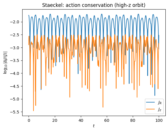
The radial action is conserved to better than a percent and the vertical action to only a fraction of a percent. This is much better than the five to ten percent errors found with the adiabatic approximation for the same orbit. Note that you can also make this plot conveniently using the Orbit interface to the actions, which automatically uses the Staeckel approximation for the action calculation:

# Initialize new Orbits all along the integrated orbit, then compute the actions
# because actions are only computed at the initial condition for the orbit interface
o_along_orbit = o(ts)
jrs = o_along_orbit.jr(pot=MWPotential2014, delta=0.4)
jzs = o_along_orbit.jz(pot=MWPotential2014, delta=0.4)

plt.plot(ts, numpy.log10(numpy.fabs((jrs - numpy.mean(jrs)) / numpy.mean(jrs))))
plt.plot(ts, numpy.log10(numpy.fabs((jzs - numpy.mean(jzs)) / numpy.mean(jzs))))
plt.xlabel(r"$t$")
plt.ylabel(r"$\log_{10}|\Delta J / \langle J \rangle|$")
plt.legend([r"$J_R$", r"$J_z$"])
plt.title("Staeckel: action conservation (high-z orbit)");

Checking that angles increase linearly

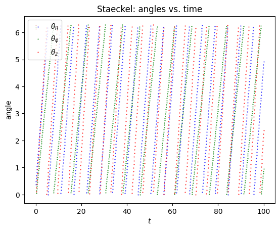
We can also verify that the angles increase linearly along the orbit:

o2 = Orbit([1.0, 0.1, 1.1, 0.0, 0.25, 0.0])
o2.integrate(ts, MWPotential2014)

jfa = aAS.actionsFreqsAngles(
    o2.R(ts), o2.vR(ts), o2.vT(ts), o2.z(ts), o2.vz(ts), o2.phi(ts)
)

plt.plot(ts, jfa[6], "b.", ms=1)
plt.plot(ts, jfa[7], "g.", ms=1)
plt.plot(ts, jfa[8], "r.", ms=1)
plt.xlabel(r"$t$")
plt.ylabel(r"angle")
plt.legend([r"$\theta_R$", r"$\theta_\phi$", r"$\theta_z$"])
plt.title("Staeckel: angles vs. time");

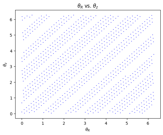
We can also look at the angle-angle plane:

plt.plot(jfa[6], jfa[8], "b.", ms=1)
plt.xlabel(r"$\theta_R$")
plt.ylabel(r"$\theta_z$")
plt.title(r"$\theta_R$ vs. $\theta_z$");

Grid-based interpolation: actionAngleStaeckelGrid

For applications requiring many evaluations (e.g., distribution functions), you can set up a grid-based interpolation that precomputes actions on a grid and interpolates. Because this is a fully three-dimensional grid, setting up the grid takes longer than for the adiabatic method, but evaluations are significantly faster afterwards:

from galpy.actionAngle import actionAngleStaeckelGrid

aASG = actionAngleStaeckelGrid(
    pot=MWPotential2014, delta=0.4, c=True, nE=51, npsi=51, nLz=61
)

Compare the grid-based and direct calculations:

# Same interface as actionAngleStaeckel
jr_direct, _, jz_direct = aAS(o.R(), o.vR(), o.vT(), o.z(), o.vz())
jr_grid, _, jz_grid = aASG(o.R(), o.vR(), o.vT(), o.z(), o.vz())

print(
    f"J_R: direct = {jr_direct.item():.6f}, grid = {jr_grid.item():.6f}, difference = {jr_grid.item() - jr_direct.item():.6f}"
)
print(
    f"J_z: direct = {jz_direct.item():.6f}, grid = {jz_grid.item():.6f}, difference = {jz_grid.item() - jz_direct.item():.6f}"
)

J_R: direct = 0.019222, grid = 0.019221, difference = -0.000001
J_z: direct = 0.015277, grid = 0.015023, difference = -0.000254

The grid-based interpolation gives a significant speed-up over even the direct C implementation (up to about 25 times for large arrays). The speed-up is especially significant for complex potentials.

Speed-up with C and fixed_quad

The actionAngleStaeckel calculations can be sped up in two ways:

1. Using Gaussian quadrature with fixed_quad=True (about 10x speed-up)

2. Using the C implementation with c=True (additional 15x speed-up for arrays)

For MWPotential2014, the overall speed-up from Python without fixed_quad to C is very significant, and the grid-based version is faster still.

Using the Orbit interface

The simplest way to use the Staeckel approximation is through the Orbit class. After integrating an orbit (or even without integrating), you can compute actions, frequencies, eccentricity, and other orbital parameters directly. The delta parameter is auto-determined from the potential when not specified.

This is the recommended approach for most use cases:

# Using the Orbit interface -- no need to set up actionAngleStaeckel manually
o_orb = Orbit([1.0, 0.1, 1.1, 0.0, 0.25, 0.0])

# Actions (delta is auto-determined from the potential)
print("J_R  =", o_orb.jr(pot=MWPotential2014))
print("L_z  =", o_orb.jp(pot=MWPotential2014))
print("J_z  =", o_orb.jz(pot=MWPotential2014))

# Frequencies
print("Omega_R   =", o_orb.Or(pot=MWPotential2014))
print("Omega_phi =", o_orb.Op(pot=MWPotential2014))
print("Omega_z   =", o_orb.Oz(pot=MWPotential2014))

# Orbital parameters using the Staeckel approximation (no integration needed)
print("Eccentricity:", o_orb.e(analytic=True, pot=MWPotential2014, type="staeckel"))
print("Apocenter:", o_orb.rap(analytic=True, pot=MWPotential2014, type="staeckel"))
print("Pericenter:", o_orb.rperi(analytic=True, pot=MWPotential2014, type="staeckel"))
print("zmax:", o_orb.zmax(analytic=True, pot=MWPotential2014, type="staeckel"))

J_R  = 0.018194068810168045
L_z  = 1.1
J_z  = 0.015401555843492853
Omega_R   = 1.1132510099651385
Omega_phi = 0.8316073031034159
Omega_z   = 1.3979171640553745
Eccentricity: 0.15606311338037263
Apocenter: 1.3449641120910967
Pericenter: 0.9818363826645405
zmax: 0.16222777310650005

Example: Lindblad resonances in the Solar neighborhood with Gaia

As a real-world application, we use the Staeckel approximation to compute actions for a large sample of nearby stars from Gaia DR3 and look for evidence of orbital resonances in the \((L_z, \sqrt{J_R})\) plane, following Trick, Coronado & Rix (2019).

We select stars within 200 pc (parallax > 5 mas) with good parallaxes (better than 5% precision) and radial velocities in Gaia DR3:

Warning

This cell queries the ESA Gaia archive, which can be slow or temporarily unavailable. If that query fails, we automatically fall back to the same Gaia DR3 catalog served by the CDS VizieR TAP endpoint via pyvo.

import os

from astropy.table import Table

from galpy.util import plot as galpy_plot

# Cache the query result locally so re-runs of this notebook don't repeat
# the multi-minute Gaia archive download.
_gaia_cache = "gaia_dr3_solar_neighborhood.fits"

if os.path.exists(_gaia_cache):
    gaia = Table.read(_gaia_cache)
    print(f"Loaded {len(gaia)} stars from local cache: {_gaia_cache}")
else:
    # Primary source: ESA Gaia archive via astroquery. The archive is occasionally
    # unavailable (HTTPError), so we fall back to the same DR3 catalog served by
    # the CDS VizieR TAP endpoint via pyvo.
    try:
        from astroquery.gaia import Gaia

        query = """
        SELECT ra, dec, parallax, pmra, pmdec, radial_velocity
        FROM gaiadr3.gaia_source
        WHERE parallax > 5
          AND parallax_over_error > 20
          AND radial_velocity IS NOT NULL
          AND ruwe < 1.4
        """

        job = Gaia.launch_job_async(query)
        gaia = job.get_results()
        print(f"Downloaded {len(gaia)} stars from Gaia DR3 (ESA archive)")
    except Exception as e:
        print(
            f"ESA Gaia archive query failed ({type(e).__name__}: {e}); "
            "falling back to VizieR TAP via pyvo."
        )
        import pyvo

        cds_tap = pyvo.dal.TAPService("http://tapvizier.u-strasbg.fr/TAPVizieR/tap/")

        vizier_query = """
        SELECT RA_ICRS, DE_ICRS, Plx, pmRA, pmDE, RV
        FROM "I/355/gaiadr3"
        WHERE Plx > 5
          AND Plx / e_Plx > 20
          AND RV IS NOT NULL
          AND RUWE < 1.4
        """

        result = cds_tap.run_async(vizier_query, maxrec=1000000)
        gaia = result.to_table()
        # Rename VizieR columns to match the ESA Gaia archive schema so that the
        # remainder of the notebook can use a single set of column names.
        gaia.rename_columns(
            ["RA_ICRS", "DE_ICRS", "Plx", "pmRA", "pmDE", "RV"],
            ["ra", "dec", "parallax", "pmra", "pmdec", "radial_velocity"],
        )
        print(f"Downloaded {len(gaia)} stars from Gaia DR3 (VizieR TAP)")

    gaia.write(_gaia_cache, format="fits", overwrite=True)

Loaded 619690 stars from local cache: gaia_dr3_solar_neighborhood.fits

Initialize orbits from the observed coordinates and compute actions using the Staeckel approximation with delta=0.45 (following Trick et al. 2019):

from galpy.orbit import Orbit

vxvv = numpy.column_stack(
    [
        numpy.array(gaia["ra"], dtype=float),
        numpy.array(gaia["dec"], dtype=float),
        1.0 / numpy.array(gaia["parallax"], dtype=float),  # kpc
        numpy.array(gaia["pmra"], dtype=float),
        numpy.array(gaia["pmdec"], dtype=float),
        numpy.array(gaia["radial_velocity"], dtype=float),
    ]
)

orbits = Orbit(vxvv, radec=True, ro=8.0, vo=220.0)
jr = orbits.jr(pot=MWPotential2014, analytic=True, type="staeckel", delta=0.45)
lz = orbits.Lz()
Lz0 = 8.0 * 220.0  # kpc km/s, solar circular angular momentum

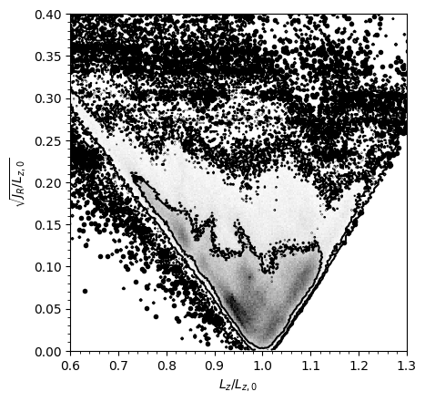
Plotting \(\sqrt{J_R}\) vs. \(L_z\) (following Trick et al. 2019; the square root emphasizes structure at low \(J_R\)) reveals clear overdensities and ridge-like features that are the signatures of orbital resonances (Sellwood 2010). The dominant feature is the Outer Lindblad Resonance of the Galactic bar:

galpy_plot.scatterplot(
    lz / Lz0,
    numpy.sqrt(jr / Lz0),
    "k.",
    xlabel=r"$L_z / L_{z,0}$",
    ylabel=r"$\sqrt{J_R / L_{z,0}}$",
    xrange=[0.6, 1.3],
    yrange=[0.0, 0.4],
);

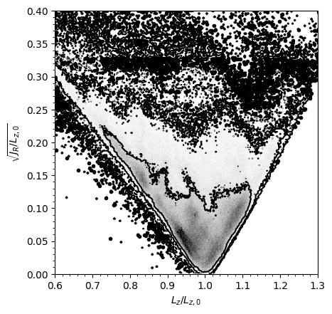
These features are robust to the choice of potential model. For example, using a LogarithmicHaloPotential (with delta=0.01 since this potential is nearly spherical) gives a very similar picture:

from galpy.potential import LogarithmicHaloPotential

loglp = LogarithmicHaloPotential(normalize=1.0)
jr_log = orbits.jr(pot=loglp, analytic=True, type="staeckel", delta=0.01)

galpy_plot.scatterplot(
    lz / Lz0,
    numpy.sqrt(jr_log / Lz0),
    "k.",
    xlabel=r"$L_z / L_{z,0}$",
    ylabel=r"$\sqrt{J_R / L_{z,0}}$",
    xrange=[0.6, 1.3],
    yrange=[0.0, 0.4],
);

The persistence of the overdensities and ridge features across different potentials is a strong indication that they are real dynamical features rather than artifacts of the potential model.