This page was generated from a Jupyter notebook. You can download it here.

Introduction to Action-Angle Coordinates

Action-angle coordinates \((\mathbf{J}, \boldsymbol{\theta})\) are canonical coordinates for integrable Hamiltonian systems in which the actions \(\mathbf{J}\) are constants of motion and the angles \(\boldsymbol{\theta}\) increase linearly with time at rates given by the frequencies \(\boldsymbol{\Omega}\).

For an axisymmetric potential, the three actions are:

• \(J_R\): radial action (related to the radial oscillation amplitude)

• \(L_z\): z-component of angular momentum (azimuthal action)

• \(J_z\): vertical action (related to the vertical oscillation amplitude)

The corresponding frequencies are \(\Omega_R\), \(\Omega_\phi\), and \(\Omega_z\).

galpy supports both forward transformations \((\mathbf{x}, \mathbf{v}) \to (\mathbf{J}, \boldsymbol{\theta}, \boldsymbol{\Omega})\) and inverse transformations \((\mathbf{J}, \boldsymbol{\theta}) \to (\mathbf{x}, \mathbf{v})\).

%matplotlib inline
import numpy
import matplotlib.pyplot as plt
import warnings

warnings.filterwarnings("ignore", category=RuntimeWarning)
warnings.filterwarnings("ignore", category=UserWarning)

Using the Orbit interface

The simplest way to compute actions, frequencies, and angles is through the Orbit class. After integrating an orbit, you can call methods like o.jr(), o.jp(), o.jz() for actions, o.Or(), o.Op(), o.Oz() for frequencies, and o.wr(), o.wp(), o.wz() for angles. Or you can call these without first integrating the orbit, but specifying the potential pot= (the orbit integration itself is not used to compute the actions, frequencies, or angles).

These methods automatically select an appropriate action-angle calculator based on the potential.

from galpy.orbit import Orbit
from galpy.potential import MWPotential2014

o = Orbit([1.0, 0.1, 1.1, 0.0, 0.05, 0.0])

# Actions
print("J_R  =", o.jr(pot=MWPotential2014))
print("L_z  =", o.jp(pot=MWPotential2014))
print("J_z  =", o.jz(pot=MWPotential2014))

J_R  = 0.01360159056118068
L_z  = 1.1
J_z  = 0.0004641949775060394

Frequencies tell us the rate at which angles increase:

# Frequencies
print("Omega_R   =", o.Or(pot=MWPotential2014))
print("Omega_phi =", o.Op(pot=MWPotential2014))
print("Omega_z   =", o.Oz(pot=MWPotential2014))

Omega_R   = 1.1594952066860231
Omega_phi = 0.868478513260914
Omega_z   = 2.221827947331903

And the angles at the initial time:

# Angles (at the initial time)
print("theta_R   =", o.wr(pot=MWPotential2014))
print("theta_phi =", o.wp(pot=MWPotential2014))
print("theta_z   =", o.wz(pot=MWPotential2014))

theta_R   = 0.46956828124044925
theta_phi = 6.176670459453628
theta_z   = 6.094187152519384

Isochrone potential: exact action-angle coordinates

The isochrone potential is special because it has exact analytical action-angle coordinates. This makes it ideal for testing.

from galpy.potential import IsochronePotential
from galpy.actionAngle import actionAngleIsochrone, actionAngleIsochroneInverse

ip = IsochronePotential(b=0.9, normalize=1.0)
aAI = actionAngleIsochrone(ip=ip)
aAII = actionAngleIsochroneInverse(ip=ip)

Direct usage of actionAngleIsochrone

We can compute actions, frequencies, and angles by passing phase-space coordinates directly to the actionsFreqsAngles method:

# Phase-space point: R, vR, vT, z, vz, phi
R, vR, vT, z, vz, phi = 1.0, 0.1, 1.1, 0.0, 0.05, 0.0

jr, jphi, jz, Or, Op, Oz, wr, wp, wz = aAI.actionsFreqsAngles(R, vR, vT, z, vz, phi)
print(f"J_R = {jr[0]:.6f}")
print(f"L_z = {jphi[0]:.6f}")
print(f"J_z = {jz[0]:.6f}")
print(f"Omega_R = {Or[0]:.6f}, Omega_phi = {Op[0]:.6f}, Omega_z = {Oz[0]:.6f}")
print(f"theta_R = {wr[0]:.6f}, theta_phi = {wp[0]:.6f}, theta_z = {wz[0]:.6f}")

J_R = 0.007866
L_z = 1.100000
J_z = 0.001136
Omega_R = 1.559710, Omega_phi = 0.949474, Omega_z = 0.949474
theta_R = 0.600400, theta_phi = 6.213239, theta_z = 6.213239

If you only need the actions (not the frequencies or angles), use the __call__ method which is faster:

jr, jphi, jz = aAI(R, vR, vT, z, vz, phi)
print(f"J_R = {jr[0]:.6f}, L_z = {jphi[0]:.6f}, J_z = {jz[0]:.6f}")

J_R = 0.007866, L_z = 1.100000, J_z = 0.001136

Generally, for the forward transformations \((\mathbf{x}, \mathbf{v}) \to (\mathbf{J}, \boldsymbol{\theta}, \boldsymbol{\Omega})\), actions, frequencies, and angles can typically be calculated using these three methods:

• __call__: returns the actions

• actionsFreqs: returns the actions and the frequencies

• actionsFreqsAngles: returns the actions, frequencies, and angles

Verifying action conservation along an orbit

Actions should be conserved along an orbit. Let’s integrate an orbit in the isochrone potential and verify this:

o = Orbit([1.0, 0.1, 1.1, 0.0, 0.05, 0.0])
ts = numpy.linspace(0.0, 50.0, 1001)
o.integrate(ts, ip)

# Compute actions at each timestep
Rs = o.R(ts)
vRs = o.vR(ts)
vTs = o.vT(ts)
zs = o.z(ts)
vzs = o.vz(ts)
phis = o.phi(ts)

jrs, jphis, jzs = aAI(Rs, vRs, vTs, zs, vzs, phis)

plt.plot(ts, jrs / jrs[0], label=r"$J_R / J_R(0)$")
plt.plot(ts, jzs / jzs[0], label=r"$J_z / J_z(0)$")
plt.xlabel(r"$t$")
plt.ylabel(r"$J / J(0)$")
plt.legend()
plt.title("Action conservation in the isochrone potential");

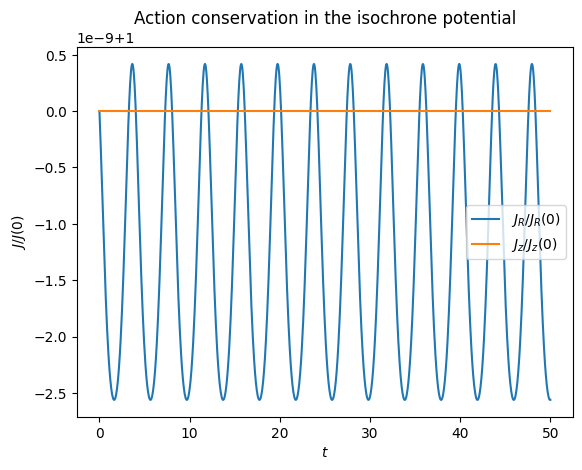
The actions are very well conserved, confirming the exactness of the isochrone action-angle calculation.

Exact inverse transform with actionAngleIsochroneInverse

The isochrone potential is also special because its inverse transformation is analytical. In general, inverse action-angle objects provide these methods:

• __call__: returns the phase-space coordinates

• xvFreqs: returns the phase-space coordinates and the frequencies

• Freqs: returns the frequencies for the specified actions

For the isochrone case, we can use actionAngleIsochroneInverse to map a set of actions and angles back to (R, vR, vT, z, vz, phi) and check that the forward and inverse transformations are consistent.

angles = numpy.array([wr[0], wp[0], wz[0]])
R_inv, vR_inv, vT_inv, z_inv, vz_inv, phi_inv = aAII(
    jr[0], jphi[0], jz[0], angles[:1], angles[1:2], angles[2:]
)
R_xv, vR_xv, vT_xv, z_xv, vz_xv, phi_xv, Or_inv, Op_inv, Oz_inv = aAII.xvFreqs(
    jr[0], jphi[0], jz[0], angles[:1], angles[1:2], angles[2:]
)
dphi = ((phi_inv[0] - phi + numpy.pi) % (2.0 * numpy.pi)) - numpy.pi
print(
    "Recovered phase-space point:",
    f"R={R_inv[0]:.6f}, vR={vR_inv[0]:.6f}, vT={vT_inv[0]:.6f}, ",
    f"z={z_inv[0]:.6f}, vz={vz_inv[0]:.6f}, phi={phi_inv[0]:.6f}",
)
print(
    "Absolute differences:",
    numpy.abs(
        [
            R_inv[0] - R,
            vR_inv[0] - vR,
            vT_inv[0] - vT,
            z_inv[0] - z,
            vz_inv[0] - vz,
            dphi,
        ]
    ),
)
print(
    "xvFreqs matches __call__:",
    numpy.allclose(
        [R_inv[0], vR_inv[0], vT_inv[0], z_inv[0], vz_inv[0], phi_inv[0]],
        [R_xv[0], vR_xv[0], vT_xv[0], z_xv[0], vz_xv[0], phi_xv[0]],
    ),
)
print("Frequencies from xvFreqs:", (Or_inv, Op_inv, Oz_inv))
print("Frequencies from Freqs:", aAII.Freqs(jr[0], jphi[0], jz[0]))

Recovered phase-space point: R=1.000000, vR=0.100000, vT=1.100000,  z=-0.000000, vz=0.050000, phi=6.283185
Absolute differences: [2.22044605e-16 9.71445147e-16 2.22044605e-16 5.14517738e-17
 1.11022302e-16 0.00000000e+00]
xvFreqs matches __call__: True
Frequencies from xvFreqs: (np.float64(1.5597097975694187), np.float64(0.9494736851422911), np.float64(0.9494736851422911))
Frequencies from Freqs: (np.float64(1.5597097975694187), np.float64(0.9494736851422911), np.float64(0.9494736851422911))

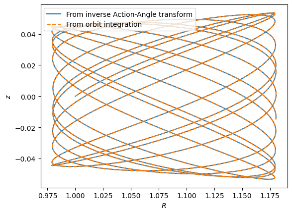
We can also compute an entire orbit with the inverse transform by specifying a time array and using the fact that angles increase linearly with time:

ts = numpy.linspace(0.0, 50.0, 1001)
rates = numpy.array([Or[0], Op[0], Oz[0]])
angles_t = angles[None, :] + ts[:, None] * rates[None, :]
R_inv, vR_inv, vT_inv, z_inv, vz_inv, phi_inv = aAII(
    jr[0], jphi[0], jz[0], angles_t[:, 0], angles_t[:, 1], angles_t[:, 2]
)
# Also integrate an orbit to compare
o = Orbit([R_inv[0], vR_inv[0], vT_inv[0], z_inv[0], vz_inv[0], phi_inv[0]])
o.integrate(ts, ip)
R_xv, vR_xv, vT_xv, z_xv, vz_xv, phi_xv = (
    o.R(ts),
    o.vR(ts),
    o.vT(ts),
    o.z(ts),
    o.vz(ts),
    o.phi(ts),
)
plt.plot(R_inv, z_inv, label="From inverse Action-Angle transform")
plt.plot(R_xv, z_xv, label="From orbit integration", ls="--")
plt.xlabel(r"$R$")
plt.ylabel(r"$z$")
plt.legend(loc="upper left");

Spherical potentials: actionAngleSpherical

For any spherical potential, actions can be computed exactly using actionAngleSpherical, which uses numerical integration of the radial and vertical oscillations.

For non-spherical potentials, see the Adiabatic Approximation, Staeckel Approximation, and Isochrone Approximation methods. For the inverse transformation (actions to coordinates), see actionAngleTorus.

from galpy.potential import LogarithmicHaloPotential
from galpy.actionAngle import actionAngleSpherical

# Spherical logarithmic halo (q=1)
lp = LogarithmicHaloPotential(normalize=1.0, q=1.0)
aAS = actionAngleSpherical(pot=lp)

jr, jphi, jz = aAS(1.0, 0.1, 1.1, 0.0, 0.05, 0.0)
print(f"J_R = {jr[0]:.6f}, L_z = {jphi[0]:.6f}, J_z = {jz[0]:.6f}")

J_R = 0.011687, L_z = 1.100000, J_z = 0.001136

The full set of actions, frequencies, and angles:

# Full actions, frequencies, and angles
jr, jphi, jz, Or, Op, Oz, wr, wp, wz = aAS.actionsFreqsAngles(
    1.0, 0.1, 1.1, 0.0, 0.05, 0.0
)
print(f"Omega_R = {Or[0]:.4f}, Omega_phi = {Op[0]:.4f}, Omega_z = {Oz[0]:.4f}")

Omega_R = 1.2669, Omega_phi = 0.8947, Omega_z = 0.8947

Verifying action conservation with actionAngleSpherical

Let’s verify that actions are conserved along an orbit in the spherical logarithmic potential:

o_sph = Orbit([1.0, 0.1, 1.1, 0.0, 0.05, 0.0])
ts_sph = numpy.linspace(0.0, 50.0, 1001)
o_sph.integrate(ts_sph, lp)

jrs_sph, jphis_sph, jzs_sph = aAS(
    o_sph.R(ts_sph),
    o_sph.vR(ts_sph),
    o_sph.vT(ts_sph),
    o_sph.z(ts_sph),
    o_sph.vz(ts_sph),
    o_sph.phi(ts_sph),
)

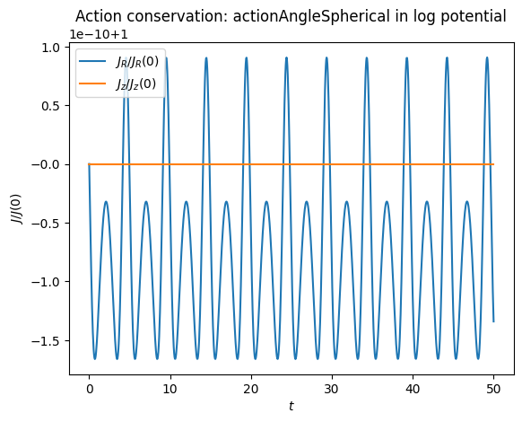
plt.plot(ts_sph, jrs_sph / jrs_sph[0], label=r"$J_R / J_R(0)$")
plt.plot(ts_sph, jzs_sph / jzs_sph[0], label=r"$J_z / J_z(0)$")
plt.xlabel(r"$t$")
plt.ylabel(r"$J / J(0)$")
plt.legend()
plt.title("Action conservation: actionAngleSpherical in log potential");