This page was generated from a Jupyter notebook. You can download it here.

Action-Angle Coordinates: Inverse Transformations (actionAngleTorus)

The actionAngleTorus class performs the inverse transformation: given actions and angles, it computes phase-space coordinates \((\mathbf{x}, \mathbf{v})\). It uses an interface to the TorusMapper code (Binney & McMillan 2016).

This is useful for:

• Setting up initial conditions with specific actions

• Computing orbital tori

• Mapping the orbital building blocks of galaxies

Currently, this is limited to axisymmetric potentials.

For the forward transformation (coordinates to actions), see the Introduction, the Staeckel Approximation, or the Isochrone Approximation.

%matplotlib inline
import numpy
import matplotlib.pyplot as plt
from galpy.potential import MWPotential2014
from galpy.orbit import Orbit
import warnings

warnings.filterwarnings("ignore", category=RuntimeWarning)
warnings.filterwarnings("ignore", category=UserWarning)

Setup

The actionAngleTorus class requires the Torus C extension. If you see a RuntimeError below, you need to install the Torus module. See the galpy installation instructions for details on how to build galpy with Torus support.

from galpy.actionAngle import actionAngleTorus

try:
    aAT = actionAngleTorus(pot=MWPotential2014)
except RuntimeError:
    raise RuntimeError(
        "actionAngleTorus requires the Torus code. See the installation instructions."
    )

Computing frequencies

Given a set of actions \((J_R, L_z, J_z)\), we first compute the frequencies using the Freqs method. This returns \((\Omega_R, \Omega_\phi, \Omega_z, \mathrm{err})\), where the last entry is the exit code of the TorusMapper (printed as a warning when non-zero):

jr_val, lz_val, jz_val = 0.1, 1.1, 0.2
Om = aAT.Freqs(jr_val, lz_val, jz_val)
print(f"Omega_R = {Om[0]:.6f}, Omega_phi = {Om[1]:.6f}, Omega_z = {Om[2]:.6f}")

Omega_R = 0.809412, Omega_phi = 0.584322, Omega_z = 0.654556

Forward transform: actions+angles to phase-space coordinates

The basic usage is aAT(jr, lz, jz, angler, anglephi, anglez), which returns [R, vR, vT, z, vz, phi].

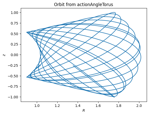
Computing an orbit from action-angle coordinates

We can compute a set of angles that fall along an orbit as \(\boldsymbol{\theta}(t) = \boldsymbol{\theta}_0 + \boldsymbol{\Omega} t\):

jr_val, lz_val, jz_val = 0.1, 1.1, 0.2
times = numpy.linspace(0.0, 100.0, 10001)
init_angle = numpy.array([1.0, 2.0, 3.0])
angles = numpy.tile(init_angle, (len(times), 1)) + Om[:3] * numpy.tile(times, (3, 1)).T

RvR, _, _, _, _ = aAT.xvFreqs(
    jr_val, lz_val, jz_val, angles[:, 0], angles[:, 1], angles[:, 2]
)

plt.plot(RvR[:, 0], RvR[:, 3])
plt.xlabel(r"$R$")
plt.ylabel(r"$z$")
plt.title("Orbit from actionAngleTorus")

Text(0.5, 1.0, 'Orbit from actionAngleTorus')

Comparison with direct orbit integration

We can compare this to a numerically integrated orbit starting from the same initial conditions:

orb = Orbit(RvR[0])
orb.integrate(times, MWPotential2014)

plt.plot(RvR[:, 0], RvR[:, 3], label="Torus")
plt.plot(orb.R(times), orb.z(times), "--", label="Orbit integration")
plt.xlabel(r"$R$")
plt.ylabel(r"$z$")
plt.legend()
plt.title("Torus vs. direct orbit integration")

Text(0.5, 1.0, 'Torus vs. direct orbit integration')

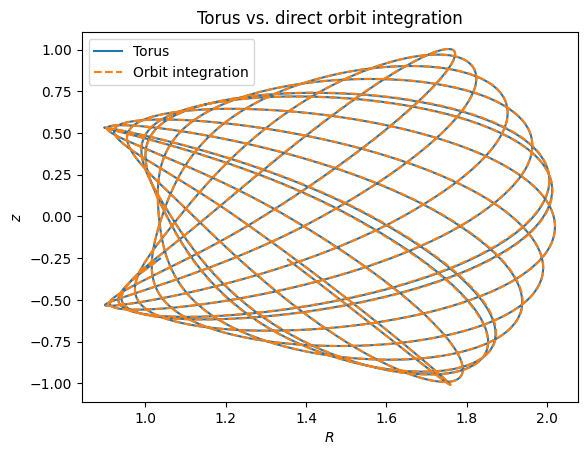
The two orbits are exactly the same.

The xvFreqs method

The xvFreqs method returns both phase-space coordinates and frequencies. The frequency is always computed and returned because it can be obtained at zero cost. The return value is (RvR, OR, Op, Oz, err) where RvR has shape (ntimes, 6) with columns (R, vR, vT, z, vz, phi):

angler = numpy.linspace(0.0, 2.0 * numpy.pi, 101)
anglephi = numpy.zeros(101)
anglez = numpy.zeros(101)

result = aAT.xvFreqs(jr_val, lz_val, jz_val, angler, anglephi, anglez)
RvR_slice = result[0]
OR, Op, Oz = result[1], result[2], result[3]

print(f"Omega_R = {OR:.6f}, Omega_phi = {Op:.6f}, Omega_z = {Oz:.6f}")

Omega_R = 0.809412, Omega_phi = 0.584322, Omega_z = 0.654556

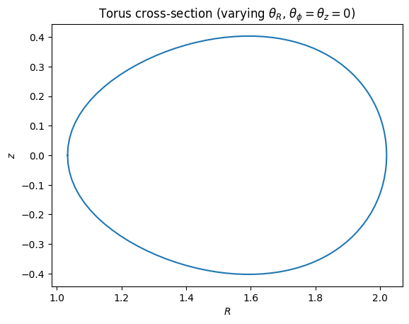
Orbital torus cross-section

By varying one angle while holding the others fixed, we can visualize a cross-section of the orbital torus:

plt.plot(RvR_slice[:, 0], RvR_slice[:, 3])
plt.xlabel(r"$R$")
plt.ylabel(r"$z$")
plt.title(r"Torus cross-section (varying $\theta_R$, $\theta_\phi = \theta_z = 0$)")

Text(0.5, 1.0, 'Torus cross-section (varying $\\theta_R$, $\\theta_\\phi = \\theta_z = 0$)')

Mapping a full torus

We do not have to follow the path of an orbit to map the entire orbital torus. By sampling random angles uniformly in \([0, 2\pi]\), we can directly visualize where the orbit spends most of its time:

numpy.random.seed(1)
nangles = 200001
angler_rand = numpy.random.uniform(size=nangles) * 2.0 * numpy.pi
anglep_rand = numpy.random.uniform(size=nangles) * 2.0 * numpy.pi
anglez_rand = numpy.random.uniform(size=nangles) * 2.0 * numpy.pi

RvR_torus, _, _, _, _ = aAT.xvFreqs(
    jr_val, lz_val, jz_val, angler_rand, anglep_rand, anglez_rand
)

plt.plot(RvR_torus[:, 0], RvR_torus[:, 3], ",", alpha=0.02)
plt.xlabel(r"$R$")
plt.ylabel(r"$z$")
plt.title("Full orbital torus")

Text(0.5, 1.0, 'Full orbital torus')

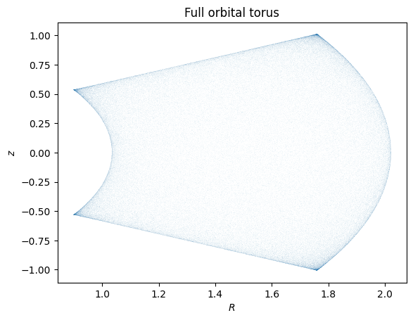
This directly shows where the orbit spends most of its time.

actionAngleTorus also has additional methods for computing Hessians and Jacobians of the transformation between action-angle and configuration space coordinates. See the action-angle API documentation for details.