This page was generated from a Jupyter notebook. You can download it here.

Action-Angle Coordinates: Orbit Integration-based (IsochroneApprox)

The actionAngleIsochroneApprox method (Bovy 2014) computes actions by integrating the orbit. By employing an auxiliary isochrone potential, actionAngleIsochroneApprox calculates action-angle variables by arithmetic operations on the actions and angles calculated in the auxiliary potential along an orbit (integrated in the true potential). Full details can be found in Appendix A of Bovy (2014). This method is completely general for any static potential and can calculate actions to any desired precision for any orbit, including orbits in triaxial potentials.

The adiabatic and Staeckel approximations are good for stars on close-to-circular orbits, but they break down for more eccentric orbits (specifically, orbits for which the radial and/or vertical action is of a similar magnitude as the angular momentum). The actionAngleIsochroneApprox method overcomes this limitation.

%matplotlib inline
import numpy
import matplotlib.pyplot as plt
from galpy.potential import LogarithmicHaloPotential
from galpy.orbit import Orbit
import warnings

warnings.filterwarnings("ignore", category=RuntimeWarning)
warnings.filterwarnings("ignore", category=UserWarning)

Setup

We set up the method for a flattened logarithmic potential. The key parameter is b, the scale parameter of the auxiliary isochrone potential (this can also be specified as an IsochronePotential instance through ip=):

from galpy.actionAngle import actionAngleIsochroneApprox

lp = LogarithmicHaloPotential(normalize=1.0, q=0.9)
aAIA = actionAngleIsochroneApprox(pot=lp, b=0.8)

Estimating the optimal b parameter

The estimateBIsochrone function estimates a good scale parameter for the auxiliary isochrone potential. When given multiple \(R\) and \(z\) values (e.g., from an orbit), it returns the minimum, median, and maximum \(b\):

from galpy.actionAngle import estimateBIsochrone

# An orbit similar to GD-1
obs = numpy.array(
    [1.56148083, 0.35081535, -1.15481504, 0.88719443, -0.47713334, 0.12019596]
)

o = Orbit(obs)
ts = numpy.linspace(0.0, 100.0, 1001)
o.integrate(ts, lp)

bmin, bmed, bmax = estimateBIsochrone(lp, o.R(ts), o.z(ts))
print(f"b_min = {bmin:.4f}, b_median = {bmed:.4f}, b_max = {bmax:.4f}")

b_min = 0.7807, b_median = 1.2266, b_max = 1.4899

Experience shows that a scale parameter somewhere in this range makes sure that the angles go through the full \([0, 2\pi]\) range, which is required for the method. If they do not, galpy will raise a warning.

Computing actions

Note that actionAngleIsochroneApprox returns arrays even for single inputs:

jr, jphi, jz = aAIA(*obs)
print(f"J_R = {jr[0]:.6f}, L_z = {jphi[0]:.6f}, J_z = {jz[0]:.6f}")

J_R = 0.166050, L_z = -1.803222, J_z = 0.507044

Convergence: the importance of choosing a good b

An essential requirement is that the angles calculated in the auxiliary potential go through the full range \([0, 2\pi]\). If this is not the case, galpy will raise a warning and the actions will not be reliable.

Let’s see what happens with a poor choice of b:

import warnings

aAIA_bad = actionAngleIsochroneApprox(pot=lp, b=1.5)
with warnings.catch_warnings(record=True) as w:
    warnings.simplefilter("always")
    jr_bad, _, jz_bad = aAIA_bad(*obs)
    if w:
        print(f"Warning: {w[0].message}")
print(f"J_R (b=1.5) = {jr_bad[0]:.6f} vs J_R (b=0.8) = {jr[0]:.6f}")

Warning: Using C implementation to integrate orbits
J_R (b=1.5) = 0.011201 vs J_R (b=0.8) = 0.166050

The plot() method: inspecting convergence

We can inspect how the angles increase and how the actions converge using the aAIA.plot function.

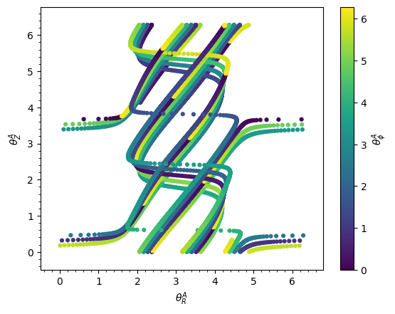
First, let’s look at the poor b=1.5 case. The radial vs. vertical angle in the auxiliary potential shows very non-linear behavior:

aAIA_bad.plot(*obs, type="araz");

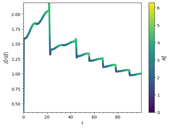
The convergence of \(J_R\) is also very slow:

aAIA_bad.plot(*obs, type="jr");

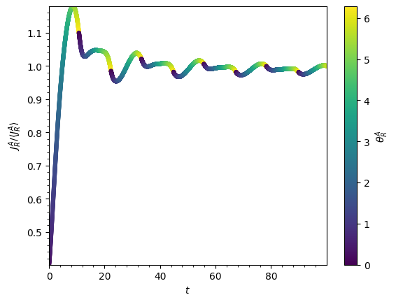
Now compare with the good b=0.8 choice, which shows quick convergence:

aAIA.plot(*obs, type="jr");

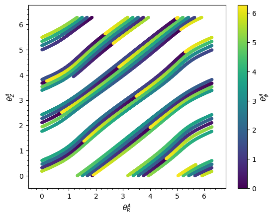
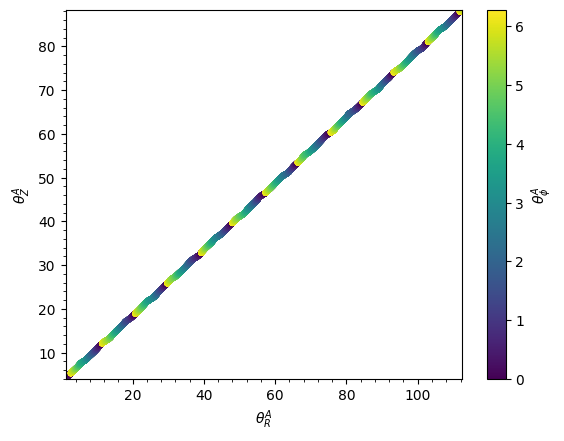
The angle-angle plot with b=0.8 shows much more linear behavior:

aAIA.plot(*obs, type="araz");

Deperioding the angles

We can remove the periodic behavior from the angles using deperiod=True, which clearly shows that they increase close-to-linearly with time:

aAIA.plot(*obs, type="araz", deperiod=True);

Computing frequencies and angles

With a good auxiliary potential, we can also compute frequencies and angles. The maxn argument controls the maximum \(n\) for which sinusoidal wiggles are removed:

result = aAIA.actionsFreqsAngles(*obs)
print(f"J_R = {result[0][0]:.6f}, L_z = {result[1][0]:.6f}, J_z = {result[2][0]:.6f}")
print(
    f"Omega_R = {result[3][0]:.6f}, Omega_phi = {result[4][0]:.6f}, Omega_z = {result[5][0]:.6f}"
)
print(
    f"theta_R = {result[6][0]:.6f}, theta_phi = {result[7][0]:.6f}, theta_z = {result[8][0]:.6f}"
)

J_R = 0.163924, L_z = -1.803222, J_z = 0.509999
Omega_R = 0.558089, Omega_phi = -0.384758, Omega_z = 0.421997
theta_R = 0.187397, theta_phi = 0.313182, theta_z = 2.184257

Raising maxn from 3 (default) to 4 shows little change, confirming convergence:

# Raising maxn from 3 (default) to 4 shows little change, confirming convergence
result4 = aAIA.actionsFreqsAngles(*obs, maxn=4)
print(f"J_R (maxn=3) = {result[0][0]:.6f}, J_R (maxn=4) = {result4[0][0]:.6f}")
print(f"Omega_R (maxn=3) = {result[3][0]:.6f}, Omega_R (maxn=4) = {result4[3][0]:.6f}")

J_R (maxn=3) = 0.163924, J_R (maxn=4) = 0.163924
Omega_R (maxn=3) = 0.558089, Omega_R (maxn=4) = 0.558088

Triaxial potentials

This technique also works for triaxial potentials by specifying nonaxi=True. This tells the code to also use the azimuthal angle variable in the auxiliary potential (unnecessary in axisymmetric potentials where \(L_z\) is conserved):

from galpy.potential import TriaxialNFWPotential

# A MW-like triaxial halo setup (roughly NFW scale radius a~2 in galpy units)
tp = TriaxialNFWPotential(normalize=1.0, a=2.0, b=0.95, c=0.85)
aAIA_triax = actionAngleIsochroneApprox(pot=tp, b=0.8)

jr_nonaxi, jphi_nonaxi, jz_nonaxi = aAIA_triax(*obs, nonaxi=True)

print(f"Triaxial J_R (nonaxi=True) = {jr_nonaxi[0]:.6f}")
print(f"Triaxial J_phi (nonaxi=True) = {jphi_nonaxi[0]:.6f}")
print(f"Triaxial J_z (nonaxi=True) = {jz_nonaxi[0]:.6f}")

Triaxial J_R (nonaxi=True) = 0.030449
Triaxial J_phi (nonaxi=True) = -1.781219
Triaxial J_z (nonaxi=True) = 0.531130

Comparison with other methods

For a standard potential like MWPotential2014, we can compare all three forward methods:

from galpy.potential import MWPotential2014
from galpy.actionAngle import actionAngleStaeckel, actionAngleAdiabatic

aAS = actionAngleStaeckel(pot=MWPotential2014, delta=0.4, c=True)
aAA = actionAngleAdiabatic(pot=MWPotential2014, c=True)
aAIA_mw = actionAngleIsochroneApprox(pot=MWPotential2014, b=0.8)

R, vR, vT, z, vz, phi = 1.0, 0.1, 1.1, 0.0, 0.05, 0.0

jr_st, _, jz_st = aAS(R, vR, vT, z, vz)
jr_ad, _, jz_ad = aAA(R, vR, vT, z, vz)
jr_ia, _, jz_ia = aAIA_mw(R, vR, vT, z, vz, phi)

print("Method            J_R        J_z")
print(f"Staeckel:         {jr_st.item():.6f}   {jz_st.item():.6f}")
print(f"Adiabatic:        {jr_ad.item():.6f}   {jz_ad.item():.6f}")
print(f"IsochroneApprox:  {jr_ia[0]:.6f}   {jz_ia[0]:.6f}")

Method            J_R        J_z
Staeckel:         0.013636   0.000463
Adiabatic:        0.013525   0.000469
IsochroneApprox:  0.013629   0.000466