This page was generated from a Jupyter notebook. You can download it here.

Adding a New Potential in Python

galpy makes it straightforward to add new gravitational potentials. Once implemented, a new potential automatically works with all of galpy’s orbit integration, action-angle, and distribution function machinery.

The steps are:

1. Create a class that inherits from galpy.potential.Potential for conservative forces or galpy.potential.DissipativeForce for dissipative forces (see below)

2. Implement __init__ calling Potential.__init__ or DissipativeForce.__init__ with appropriate parameters

3. Implement _evaluate(self, R, z, phi=0., t=0.) for the potential value (not for dissipative forces)

4. Implement _Rforce(self, R, z, phi=0., t=0.) for the radial force

5. Implement _zforce(self, R, z, phi=0., t=0.) for the vertical force

6. Implement _phitorque(self, R, z, phi=0., t=0.) for the azimuthal torque (if non-axisymmetric)

7. Optionally implement _dens, _R2deriv, _z2deriv, _Rzderiv, etc.

%matplotlib inline
import numpy
import matplotlib.pyplot as plt
from galpy.potential import Potential
from galpy.orbit import Orbit
import warnings

warnings.filterwarnings("ignore", category=RuntimeWarning)
warnings.filterwarnings("ignore", category=UserWarning)

Example: a custom softened power-law potential

Let’s implement a softened isothermal-like potential of the form:

\[\Phi(R, z) = \frac{1}{2}\,v_0^2\,\ln(R^2 + z^2 + d^2)\]

where \(v_0\) sets the circular velocity scale and \(d\) is a softening length. This is similar to the logarithmic potential but implemented from scratch to illustrate the process.

class SoftenedLogPotential(Potential):
    """A softened logarithmic potential: Phi = 0.5 * v0^2 * ln(R^2 + z^2 + d^2)."""

    def __init__(self, amp=1.0, v0=1.0, d=0.1, ro=None, vo=None):
        """
        Initialize the potential.

        Parameters
        ----------
        amp : float
            Overall amplitude.
        v0 : float
            Velocity scale (in natural units).
        d : float
            Softening length (in natural units).
        ro, vo : float, optional
            Unit conversion parameters.
        """
        Potential.__init__(self, amp=amp, ro=ro, vo=vo)
        self._v0 = v0
        self._d = d
        self._d2 = d**2.0

    def _evaluate(self, R, z, phi=0.0, t=0.0):
        return 0.5 * self._v0**2.0 * numpy.log(R**2.0 + z**2.0 + self._d2)

    def _Rforce(self, R, z, phi=0.0, t=0.0):
        return -(self._v0**2.0) * R / (R**2.0 + z**2.0 + self._d2)

    def _zforce(self, R, z, phi=0.0, t=0.0):
        return -(self._v0**2.0) * z / (R**2.0 + z**2.0 + self._d2)

Using the new potential

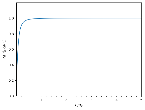
Our new potential immediately works with galpy’s plotting functions, orbit integration, and other tools.

sp = SoftenedLogPotential(v0=1.0, d=0.1)
sp.plotRotcurve(Rrange=[0.01, 5.0], grid=1001);

Orbit integration with the new potential

o = Orbit([1.0, 0.1, 1.1, 0.0, 0.1])
ts = numpy.linspace(0, 100, 10000)
o.integrate(ts, sp)
o.plot();

galpyWarning: Cannot use C integration because some of the potentials are not implemented in C (using leapfrog instead)

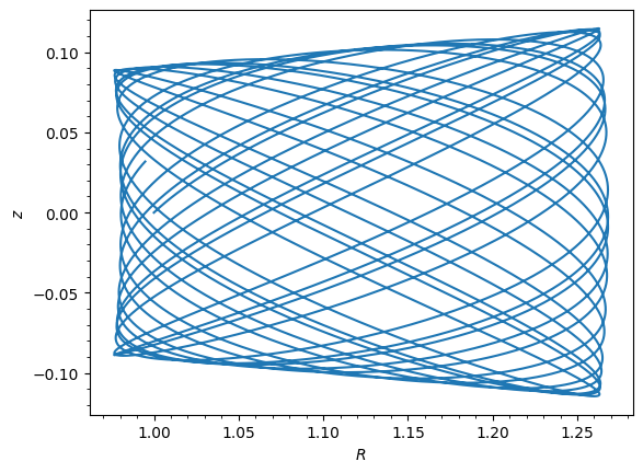
Note the warning message about not being able to use C integration, because the new potential does not have a C implementation. This means that orbit integration will be slower than for built-in potentials, but it will still work correctly.

Using normalize

The normalize keyword can be used to set the circular velocity at R=1 to a desired value. We can call normalize() after initialization.

sp_norm = SoftenedLogPotential(v0=1.0, d=0.1)
sp_norm.normalize(1.0)
print("v_circ at R=1:", sp_norm.vcirc(1.0))

v_circ at R=1: 1.0

Physical units with amp_units

To allow users to specify the amplitude of your potential in physical units (e.g., solar masses or km/s), add an amp_units class attribute. For example, for a potential whose amplitude has units of velocity squared:

class MyPotential(Potential):
    amp_units = 'velocity2'
    ...

Valid options include 'mass', 'velocity2', 'density', and 'surfacedensity'. This enables the potential to accept astropy Quantity inputs for the amplitude.

See the galpy documentation on physical units for full details.

Complete list of implementable methods

The following methods can be implemented in a custom potential class. All methods receive (self, R, z, phi=0., t=0.) as arguments. The return values should not include the amp factor – galpy handles multiplication by amp automatically.

Core methods (recommended minimum):

• _evaluate – the potential value \(\Phi(R, z, \phi, t)\) (without amp)

• _Rforce – the radial force \(-\partial\Phi/\partial R\)

• _zforce – the vertical force \(-\partial\Phi/\partial z\)

Second derivatives:

• _R2deriv – \(\partial^2\Phi/\partial R^2\)

• _z2deriv – \(\partial^2\Phi/\partial z^2\)

• _Rzderiv – \(\partial^2\Phi/\partial R\,\partial z\)

• _phi2deriv – \(\partial^2\Phi/\partial\phi^2\)

• _Rphideriv – \(\partial^2\Phi/\partial R\,\partial\phi\)

Other optional methods:

• _dens – the density \(\rho(R, z, \phi, t)\) (galpy can compute this numerically via Poisson’s equation, but an analytical form is faster and more accurate)

• _mass – the enclosed mass

• _phitorque – the azimuthal torque \(-\partial\Phi/\partial\phi\) (required for non-axisymmetric potentials)

All of these should be implemented without the amp factor.

Automatic numerical derivatives with NumericalPotentialDerivativesMixin

If you only want to implement _evaluate, _Rforce, and _zforce but still need second derivatives, you can use NumericalPotentialDerivativesMixin. This mixin automatically computes _R2deriv, _z2deriv, _Rzderiv, _phi2deriv, and _Rphideriv numerically from the forces.

To use it, inherit from both the mixin and Potential:

from galpy.potential import NumericalPotentialDerivativesMixin

class MyPotential(NumericalPotentialDerivativesMixin, Potential):
    def __init__(self, amp=1., ro=None, vo=None):
        Potential.__init__(self, amp=amp, ro=ro, vo=vo)

    def _evaluate(self, R, z, phi=0., t=0.):
        ...

    def _Rforce(self, R, z, phi=0., t=0.):
        ...

    def _zforce(self, R, z, phi=0., t=0.):
        ...

The mixin must appear before Potential in the inheritance list so its methods take precedence. The numerical derivatives are computed using finite differences and are accurate enough for most purposes.

Important class attributes

Several class attributes control how galpy interacts with your potential:

• hasC = True – set this if you also provide a C implementation of the potential (for fast orbit integration). See the Adding a New Potential in C tutorial.

• hasC_dxdv = True – set this if the C implementation also supports phase-space derivatives (for variational integration).

• hasC_dens = True – set this if the C implementation includes a density function (required for dynamical friction in this potential).

• isNonAxi = True – set this if the potential is non-axisymmetric (depends on \(\phi\)). This is False by default.

• _dim = 3 – the dimensionality of the potential. The default is 3; set to 2 for planar potentials or 1 for one-dimensional potentials.

These are set as class attributes or in __init__. For example:

class MyNonAxiPotential(Potential):
    isNonAxi = True

    def __init__(self, amp=1., ro=None, vo=None):
        Potential.__init__(self, amp=amp, ro=ro, vo=vo)
        ...

Adding wrapper potentials

galpy also supports wrapper potentials that modify or combine existing potentials. If you want to create a potential that wraps another potential (e.g., to make it time-dependent or to apply a spatial transformation), inherit from parentWrapperPotential. This base class automatically handles both 3D and 2D (planar) wrapping:

from galpy.potential.WrapperPotential import parentWrapperPotential

class MyWrapperPotential(parentWrapperPotential):
    def __init__(self, amp=1., pot=None, ro=None, vo=None):
        parentWrapperPotential.__init__(self, amp=amp, pot=pot, ro=ro, vo=vo)
        ...

The wrapped potential is available as self._pot inside your methods. See the existing wrapper potentials (e.g., DehnenSmoothWrapperPotential, SolidBodyRotationWrapperPotential) in the galpy source for examples of how to implement these.

Adding dissipative forces to the galpy framework

Dissipative (velocity-dependent) forces are implemented similarly to conservative potentials, but inherit from galpy.potential.DissipativeForce instead of galpy.potential.Potential. The main differences are:

1. You only need to implement the forces (not _evaluate, since there is no potential energy for a dissipative force).

2. The force methods take an extra keyword argument v= that gives the current velocity in cylindrical coordinates as a list [vR, vT, vz], because dissipative forces generally depend on the velocity.

The steps are:

1. Create a class that inherits from DissipativeForce.

2. In __init__, call DissipativeForce.__init__(self, amp=amp, ro=ro, vo=vo, amp_units=...) to set up the amplitude and unit system.

3. Implement the following force methods, each accepting v=None as a keyword:

   • _Rforce(self, R, z, phi=0., t=0., v=None) – the radial force

   • _phitorque(self, R, z, phi=0., t=0., v=None) – the azimuthal torque

   • _zforce(self, R, z, phi=0., t=0., v=None) – the vertical force

The v argument is a list [vR, vT, vz] in cylindrical coordinates. As for conservative potentials, the return values should not include the amp factor.

The built-in ChandrasekharDynamicalFrictionForce provides a good template to follow. There is currently no support for implementing dissipative forces in C.

For a complete worked example of adding a custom velocity-dependent force – implementing Schwarzschild precession to model the relativistic orbit of the S2 star around Sgr A* – see the Dissipative Forces tutorial.