This page was generated from a Jupyter notebook. You can download it here.

Dissipative Forces

galpy supports velocity-dependent (dissipative) forces that can be combined with regular gravitational potentials for orbit integration. These are implemented as subclasses of DissipativeForce.

Warning

Dissipative forces only work in 3D orbit integration.

%matplotlib inline
import numpy
from matplotlib import pyplot as plt
from galpy import potential
from galpy.potential import (
    MWPotential2014,
    LogarithmicHaloPotential,
    ChandrasekharDynamicalFrictionForce,
)
from galpy.orbit import Orbit
import warnings

warnings.filterwarnings("ignore", category=RuntimeWarning)
warnings.filterwarnings("ignore", category=UserWarning)

Chandrasekhar Dynamical Friction

ChandrasekharDynamicalFrictionForce implements the classical Chandrasekhar dynamical-friction formula. It requires a background potential (whose density is used to compute the local density) and the mass of the sinking object.

from astropy import units as u

# Logarithmic halo as the host
lp = LogarithmicHaloPotential(normalize=1.0, q=1.0)

# Dynamical friction from a satellite of mass 5e10 Msun
cdf = ChandrasekharDynamicalFrictionForce(
    GMs=0.5,  # satellite mass in natural units (fraction of v_0^2 * R_0)
    rhm=0.125,  # half-mass radius of the satellite
    dens=lp,  # background density from this potential
)

print(type(cdf))

<class 'galpy.potential.ChandrasekharDynamicalFrictionForce.ChandrasekharDynamicalFrictionForce'>

Now integrate an orbit with and without dynamical friction to see the effect:

# Integrate an orbit with and without dynamical friction
o_nodf = Orbit([1.5, 0.1, 0.8, 0.0, 0.0, 0.0])
o_df = Orbit([1.5, 0.1, 0.8, 0.0, 0.0, 0.0])

ts = numpy.linspace(0.0, 30.0, 10001)

# Without friction
o_nodf.integrate(ts, lp)
# With friction: combine potential + dissipative force
o_df.integrate(ts, lp + cdf)

galpyWarning: Cannot use symplectic integration because some of the included forces are dissipative (using non-symplectic integrator dopr54_c instead)
galpyWarning: Orbit integration with ChandrasekharDynamicalFrictionForce entered domain where r < minr and ChandrasekharDynamicalFrictionForce is turned off; initialize ChandrasekharDynamicalFrictionForce with a smaller minr to avoid this if you wish (but note that you want to turn it off close to the center for an object that sinks all the way to r=0, to avoid numerical instabilities)

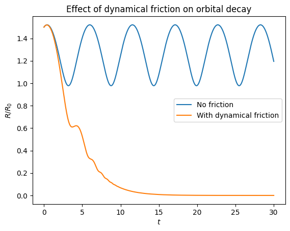
Compare the orbital radius over time:

# Compare the orbital radius over time
plt.plot(ts, o_nodf.R(ts), label="No friction")
plt.plot(ts, o_df.R(ts), label="With dynamical friction")
plt.xlabel(r"$t$")
plt.ylabel(r"$R / R_0$")
plt.legend()
plt.title("Effect of dynamical friction on orbital decay");

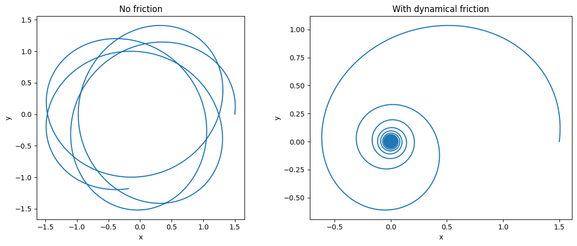
The orbit in the x-y plane clearly shows the inspiral with friction:

# Plot the orbit in x-y
fig, axes = plt.subplots(1, 2, figsize=(12, 5))
axes[0].plot(o_nodf.x(ts), o_nodf.y(ts))
axes[0].set_title("No friction")
axes[0].set_xlabel("x")
axes[0].set_ylabel("y")
axes[0].set_aspect("equal")
axes[1].plot(o_df.x(ts), o_df.y(ts))
axes[1].set_title("With dynamical friction")
axes[1].set_xlabel("x")
axes[1].set_ylabel("y")
axes[1].set_aspect("equal")
plt.tight_layout();

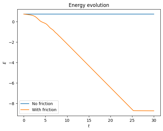
Energy dissipation

We can verify that dynamical friction removes energy from the orbit:

plt.plot(ts, o_nodf.E(ts, pot=lp), label="No friction")
plt.plot(ts, o_df.E(ts, pot=lp), label="With friction")
plt.xlabel(r"$t$")
plt.ylabel(r"$E$")
plt.legend()
plt.title("Energy evolution");

NonInertialFrameForce

galpy also provides NonInertialFrameForce for integrating orbits in non-inertial (e.g., rotating or accelerating) reference frames. This is covered in detail in the Integration and Plotting tutorial, since it is most naturally used in the context of orbit integration.

Key points:

• It adds fictitious forces (Coriolis, centrifugal, etc.)

• Specified via Omega (rotation) and/or a0 (linear acceleration)

• 3D only, like all dissipative forces

For basic potential usage, see the Introduction to Potentials.

Example: Schwarzschild precession of the S2 orbit around Sgr A*

The S2 star orbits the supermassive black hole Sgr A* at the Galactic Center on a highly eccentric orbit with a 16-year period. The GRAVITY Collaboration (2020) detected the Schwarzschild precession of S2’s orbit – the relativistic precession of the pericenter due to the GR correction to the Kepler potential. Here we reproduce this calculation using galpy by adding the first-order GR correction, which is a velocity-dependent force, to a KeplerPotential (note that it is not dissipative, just velocity-dependent).

We use rebound to convert S2’s orbital elements (semi-major axis, eccentricity, inclination, argument of pericenter, longitude of ascending node, time of pericenter) to a Cartesian position and velocity that can initialize a galpy Orbit.

import rebound
import astropy.units as u
from astropy.constants import c as c_si
from galpy.potential import KeplerPotential
from galpy.potential.DissipativeForce import DissipativeForce

c_kms = c_si.to_value(u.km / u.s)

# Sgr A* parameters
R0 = 8246.7 * u.pc
vo = 220.0 * u.km / u.s
MSgrA = 4.261e6 * u.Msun

# Set up a rebound simulation with S2's orbital elements (GRAVITY Collaboration 2020)
sim = rebound.Simulation()
sim.units = ("AU", "yr", "Msun")
sim.add(m=MSgrA.to_value(u.Msun))  # Sgr A*
sim.add(
    m=0.0,
    a=(125.058 * u.mas * R0).to_value(u.AU, equivalencies=u.dimensionless_angles()),
    e=0.884649,
    inc=(134.567 * u.deg).to_value(u.rad),
    omega=(66.263 * u.deg).to_value(u.rad),
    Omega=(228.171 * u.deg).to_value(u.rad),
    T=(8.37900 * u.yr).to_value(u.yr) - 0.35653101,  # time since 2010's apocenter
)
print(f"S2 semi-major axis = {sim.particles[1].a:.1f} AU, e = {sim.particles[1].e:.3f}")

S2 semi-major axis = 1031.3 AU, e = 0.885

Initialize a galpy Orbit from the rebound Cartesian position and velocity, then integrate it in a KeplerPotential representing Sgr A*:

pt = sim.particles[1]
# Sgr A* at the Galactic Center as the reference point
ogc = Orbit([0.0, 0.0, 0.0, 0.0, 0.0, 0.0], ro=R0, vo=vo)
ra_gc, dec_gc = ogc.ra(), ogc.dec()  # degrees (floats)


# Convert rebound Cartesian to (RA, Dec, dist, pmRA, pmDec, vlos) offsets
def make_s2_orbit():
    return Orbit(
        [
            ra_gc * u.deg
            + (pt.y * u.AU / R0).to(u.deg, equivalencies=u.dimensionless_angles()),
            dec_gc * u.deg
            + (pt.x * u.AU / R0).to(u.deg, equivalencies=u.dimensionless_angles()),
            ogc.dist() * u.kpc + pt.z * u.AU,
            ogc.pmra() * u.mas / u.yr
            + (pt.vy * u.AU / u.yr / R0).to(
                u.mas / u.yr, equivalencies=u.dimensionless_angles()
            ),
            ogc.pmdec() * u.mas / u.yr
            + (pt.vx * u.AU / u.yr / R0).to(
                u.mas / u.yr, equivalencies=u.dimensionless_angles()
            ),
            ogc.vlos() * u.km / u.s + pt.vz * u.AU / u.yr,
        ],
        radec=True,
        ro=R0,
        vo=vo,
    )


kp = KeplerPotential(amp=MSgrA, ro=R0)
times = numpy.linspace(0.0, 4.0 * 16.0455, 1001) * u.yr  # 4 orbital periods

o = make_s2_orbit()
o.integrate(times, kp)

To compute the Schwarzschild precession we implement the leading-order GR correction as a DissipativeForce (which is the galpy class for velocity-dependent forces):

\[\vec{a}_{\mathrm{SP}} = f_{\mathrm{SP}}\,\frac{GM}{c^2 r^2}\left[\left(2(\gamma+\beta)\,\frac{GM}{r} - \gamma\,v^2\right)\frac{\vec{r}}{r} + 2(1+\gamma)\,v_r\,\vec{v}\right].\]

The factor \(f_{\mathrm{SP}}\) is the “GR factor” used by GRAVITY Collaboration (2020) – \(f_{\mathrm{SP}} = 1\) corresponds to standard GR. The PPN parameters \(\gamma\) and \(\beta\) default to their GR values (\(\gamma = \beta = 1\)).

class SchwarzschildPrecessionForce(DissipativeForce):
    def __init__(self, amp=1.0, fsp=1.0, gamma=1.0, beta=1.0, ro=None, vo=None):
        DissipativeForce.__init__(self, amp=amp, ro=ro, vo=vo, amp_units="mass")
        self._fsp = fsp
        self._gamma = gamma
        self._beta = beta

    def _force_firstterm(self, r, v):
        return (
            1.0
            / (c_kms / self._vo) ** 2
            / r**3
            * (2.0 * (self._gamma + self._beta) * self._amp / r - self._gamma * v**2)
        )

    def _force_secondterm(self, r, vr):
        return 2.0 * (1.0 + self._gamma) / (c_kms / self._vo) ** 2 / r**2 * vr

    def _Rforce(self, R, z, phi=0.0, t=0.0, v=None):
        r = numpy.sqrt(R**2 + z**2)
        vr = R / r * v[0] + z / r * v[2]
        vmag = numpy.sqrt(v[0] ** 2 + v[1] ** 2 + v[2] ** 2)
        return self._fsp * (
            self._force_firstterm(r, vmag) * R + self._force_secondterm(r, vr) * v[0]
        )

    def _zforce(self, R, z, phi=0.0, t=0.0, v=None):
        r = numpy.sqrt(R**2 + z**2)
        vr = R / r * v[0] + z / r * v[2]
        vmag = numpy.sqrt(v[0] ** 2 + v[1] ** 2 + v[2] ** 2)
        return self._fsp * (
            self._force_firstterm(r, vmag) * z + self._force_secondterm(r, vr) * v[2]
        )

    def _phitorque(self, R, z, phi=0.0, t=0.0, v=None):
        r = numpy.sqrt(R**2 + z**2)
        vr = R / r * v[0] + z / r * v[2]
        return self._fsp * (self._force_secondterm(r, vr) * v[1] * R)

To make the precession clearly visible over just a few orbits, we exaggerate it with \(f_{\mathrm{SP}} = 5\). We integrate the same initial conditions in the Kepler potential plus the precession force and compare:

sp = SchwarzschildPrecessionForce(amp=MSgrA, ro=R0, fsp=5.0)

osp = make_s2_orbit()
osp.integrate(times, kp + sp)

galpyWarning: Cannot use C integration because some of the potentials are not implemented in C (using leapfrog instead)
galpyWarning: Cannot use symplectic integration because some of the included forces are dissipative (using non-symplectic integrator odeint instead)

Plot the orbit as \(\Delta\mathrm{Dec}\) vs. \(\Delta\mathrm{RA}\) relative to Sgr A*. The Newtonian Kepler orbit is a closed ellipse, while the GR orbit precesses, tracing out a rosette:

plt.figure(figsize=(5, 10))
o.plot(
    d1=f"(ra-{ra_gc})*3600",
    d2=f"(dec-{dec_gc})*3600",
    xlabel=r"$\Delta\mathrm{RA}\,(\mathrm{arcsec})$",
    ylabel=r"$\Delta\mathrm{Dec}\,(\mathrm{arcsec})$",
    label="Newtonian (Kepler)",
    gcf=True,
)
osp.plot(
    d1=f"(ra-{ra_gc})*3600",
    d2=f"(dec-{dec_gc})*3600",
    overplot=True,
    label=r"With GR precession ($f_{\mathrm{SP}}=5$)",
)
plt.plot([0], [0], "k+", ms=15, label="Sgr A*")
plt.xlim(0.075, -0.095)
plt.ylim(-0.03, 0.21)
plt.legend(fontsize=10);

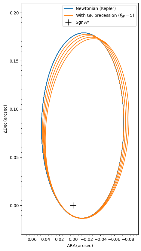
The pericenter advances by a few degrees per orbit, exactly the relativistic effect detected by GRAVITY Collaboration (2020). With the actual GR value \(f_{\mathrm{SP}} = 1\) the precession is five times smaller – still measurable with high-precision astrometry, but harder to see in a plot of just a few orbits.

Finally, let’s check that when setting \(\beta = 2(1+\gamma) = 4\) for \(\gamma = 1\) we get zero precession (a useful sanity check on the PPN form of the precession formula):

spzero = SchwarzschildPrecessionForce(amp=MSgrA, ro=R0, fsp=1.0, beta=4.0, gamma=1.0)
ozero = make_s2_orbit()
ozero.integrate(times, kp + spzero)

plt.figure(figsize=(5, 10))
o.plot(
    d1=f"(ra-{ra_gc})*3600",
    d2=f"(dec-{dec_gc})*3600",
    xlabel=r"$\Delta\mathrm{RA}\,(\mathrm{arcsec})$",
    ylabel=r"$\Delta\mathrm{Dec}\,(\mathrm{arcsec})$",
    label="Newtonian (Kepler)",
    gcf=True,
)
osp.plot(
    d1=f"(ra-{ra_gc})*3600",
    d2=f"(dec-{dec_gc})*3600",
    overplot=True,
    label=r"With GR precession ($f_{\mathrm{SP}}=5$)",
)
ozero.plot(
    d1=f"(ra-{ra_gc})*3600",
    d2=f"(dec-{dec_gc})*3600",
    overplot=True,
    ls="--",
    label=r"PPN: $\beta=2(1+\gamma)$, no precession",
)
plt.plot([0], [0], "k+", ms=15, label="Sgr A*")
plt.xlim(0.075, -0.095)
plt.ylim(-0.03, 0.21)
plt.legend(fontsize=9);

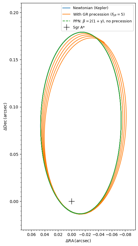
As expected, the dashed PPN curve traces the same closed ellipse as the Newtonian orbit – the choice \(\beta = 2(1+\gamma)\) exactly cancels the pericenter precession.