This page was generated from a Jupyter notebook. You can download it here.

Introduction to Potentials

galpy provides a large library of gravitational potentials. This notebook covers how to initialize potentials, evaluate them, combine them, and compute useful dynamical quantities.

See also: Potential Wrappers for time-dependent and rotating potentials, SCF and Multipole Expansions for basis-function representations, Dissipative Forces for working with dissipative forces such as dynamical friction, Milky Way Potentials for pre-built MW models, N-body snapshots for working with N-body simulation data, and Other codes for info on how to use galpy potentials with a host of other codes.

%matplotlib inline
import numpy
from matplotlib import pyplot as plt
from galpy import potential
from galpy.potential import (
    MiyamotoNagaiPotential,
    NFWPotential,
    HernquistPotential,
    LogarithmicHaloPotential,
    MWPotential2014,
)
from galpy.util import conversion
import warnings

warnings.filterwarnings("ignore", category=RuntimeWarning)
warnings.filterwarnings("ignore", category=UserWarning)

Initializing a potential

Let’s start by creating a Miyamoto-Nagai disk potential. In galpy’s natural units, velocities are normalized to the circular velocity at the Sun, and distances to the Sun’s Galactocentric radius.

mp = MiyamotoNagaiPotential(a=0.5, b=0.0375, normalize=1.0)
mp

MiyamotoNagaiPotential with internal parameters: amp=1.4632953564490085, a=0.5, b=0.0375 and physical outputs off

Evaluating potential values and forces

Evaluate the potential at (R, z) = (1, 0), i.e., the solar position in natural units. Calling the potential object directly returns the potential value:

# Potential value at (R, z) = (1, 0)
print("Phi(R=1, z=0) =", mp(1.0, 0.0))

Phi(R=1, z=0) = -1.2889062500000001

Warning

galpy potentials do not necessarily approach zero at infinity. To compute, for example, the escape velocity or whether or not an orbit is unbound, you need to take into account the value of the potential at infinity: \(v_{\mathrm{esc}}(r) = \sqrt{2[\Phi(\infty)-\Phi(r)]}\). If you want to create a potential that does go to zero at infinity, you can add a NullPotential with value equal to minus the original potential evaluated at infinity.

Tip

Potentials can be initialized and evaluated with arguments specified as astropy Quantities with units. Use the configuration parameter astropy-units = True to get output values as a Quantity. See the section on initializing potentials with physical parameters below.

To evaluate the forces, use the Rforce and zforce methods:

# Radial and vertical forces
print("F_R(R=1, z=0) =", mp.Rforce(1.0, 0.0))
print("F_z(R=1, z=0.1) =", mp.zforce(1.0, 0.1))

F_R(R=1, z=0) = -1.0
F_z(R=1, z=0.1) = -0.5194918992748312

The azimuthal torque can be computed with the phitorque method:

print("N_phi(R=1, z=0) =", mp.phitorque(1.0, 0.0))

N_phi(R=1, z=0) = 0.0

The functional interface

galpy also provides module-level functions that work on single potentials or lists of potentials:

print("evaluatePotentials:", potential.evaluatePotentials(mp, 1.0, 0.0))
print("evaluateRforces:", potential.evaluateRforces(mp, 1.0, 0.0))
print("evaluatezforces:", potential.evaluatezforces(mp, 1.0, 0.1))
print("evaluatephitorques:", potential.evaluatephitorques(mp, 1.0, 0.0))

evaluatePotentials: -1.2889062500000001
evaluateRforces: -1.0
evaluatezforces: -0.5194918992748312
evaluatephitorques: 0.0

Combining potentials

Potentials can be combined using the + operator. MWPotential2014 is a built-in composite potential with three components:

print(MWPotential2014)

CompositePotential of 3 potentials:
        PowerSphericalPotentialwCutoff with internal parameters: amp=0.029994597188218296, alpha=1.8, rc=0.2375
        MiyamotoNagaiPotential with internal parameters: amp=0.7574802019371595, a=0.375, b=0.035
        NFWPotential with internal parameters: amp=4.852230533527998, a=2.0
and physical outputs off

You can also combine potentials yourself using the + operator:

# You can also combine potentials yourself
my_pot = MiyamotoNagaiPotential(a=0.5, b=0.0375, normalize=0.6) + NFWPotential(
    a=4.5, normalize=0.35
)
print("Phi(1,0) =", my_pot(1.0, 0.0))

Phi(1,0) = -4.498828040219292

Tip

To simply adjust the amplitude of a Potential instance, you can multiply the instance by a number or divide it by a number. For example, pot = 2. * LogarithmicHaloPotential(amp=1.) is equivalent to pot = LogarithmicHaloPotential(amp=2.). This is useful if you want to quickly adjust the mass of a potential.

Physical units

The easiest way to work with physical units in galpy is to initialize potentials with the ro= and vo= parameters. When these are set, output is automatically returned in physical units. You can toggle this behavior with use_physical=True/False or with the turn_physical_on() and turn_physical_off() methods.

# Initialize MWPotential2014 with physical scales
ro, vo = 8.0, 220.0  # kpc, km/s
MWPotential2014.turn_physical_on(ro=ro, vo=vo)

# Now output is automatically in physical units
print("v_circ(R=8 kpc):", MWPotential2014.vcirc(1.0), "km/s")
print("F_R(R=8 kpc):", potential.evaluateRforces(MWPotential2014, 1.0, 0.0), "km/s/Myr")

# Toggle physical output off temporarily with use_physical=False
print(
    "\nF_R (natural units):",
    potential.evaluateRforces(MWPotential2014, 1.0, 0.0, use_physical=False),
)

# Or turn it off entirely
MWPotential2014.turn_physical_off()
print(
    "F_R after turn_physical_off:", potential.evaluateRforces(MWPotential2014, 1.0, 0.0)
)

v_circ(R=8 kpc): 220.0 km/s
F_R(R=8 kpc): -6.187408598526455 km/s/Myr

F_R (natural units): -1.0
F_R after turn_physical_off: -1.0

Alternatively, you can use the galpy.util.conversion module to manually convert from natural units to physical units. This is useful when you want to keep potentials in natural units but occasionally need a physical value:

# Manual conversion using galpy.util.conversion
F_R_nat = potential.evaluateRforces(MWPotential2014, 1.0, 0.0)
F_R_phys = F_R_nat * conversion.force_in_kmsMyr(vo, ro)
print(
    f"F_R at solar position: {F_R_nat:.4f} (natural), {F_R_phys:.4f} km/s/Myr (physical)"
)

F_R at solar position: -1.0000 (natural), -6.1874 km/s/Myr (physical)

Densities

You can evaluate the density directly or via the Poisson equation:

# Direct density evaluation
print("Density (direct):", mp.dens(1.0, 0.0))
# Via the Poisson equation
print("Density (Poisson):", mp.dens(1.0, 0.0, forcepoisson=True))

Density (direct): 1.1145444383277576
Density (Poisson): 1.1145444383277574

The functional interface also works for densities of combinations of potentials, and so does the method version:

print(
    "MWPotential2014 density at (1,0):",
    potential.evaluateDensities(MWPotential2014, 1.0, 0.0),
)

MWPotential2014 density at (1,0): 0.5750860312226487

MWPotential2014.dens(1.0, 0.0, ro=8.0, vo=220.0, use_physical=True, quantity=True)

$0.10112001 \; \mathrm{\frac{M_{\odot}}{pc^{3}}}$

DoubleExponentialDiskPotential density

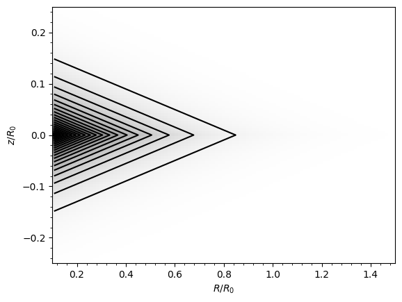
Another example: an exponential disk potential, where we can compare the analytical density to that computed via the Poisson equation and we plot the density.

from galpy.potential import DoubleExponentialDiskPotential

dp = DoubleExponentialDiskPotential(hr=1.0 / 4.0, hz=1.0 / 20.0, normalize=1.0)
# The Poisson-equation density requires numerical integration, so the agreement
# is slightly less good than for Miyamoto-Nagai, but still better than a percent:
print(
    "Relative difference:",
    (dp.dens(1.0, 0.0, forcepoisson=True) - dp.dens(1.0, 0.0)) / dp.dens(1.0, 0.0),
)
dp.plotDensity(rmin=0.1, zmax=0.25, zmin=-0.25, nrs=101, nzs=101);

Relative difference: 1.5308327107952697e-14

Flattening

We can evaluate the flattening of the potential as \(\sqrt{|z\,F_R / R\,F_Z|}\):

print("Flattening of Miyamoto-Nagai at (1, 0.125):", mp.flattening(1.0, 0.125))
print(
    "Flattening of MWPotential2014 at (1, 0.125):",
    MWPotential2014.flattening(1.0, 0.125),
)

Flattening of Miyamoto-Nagai at (1, 0.125): 0.4549542914935209
Flattening of MWPotential2014 at (1, 0.125): 0.6123167530565863

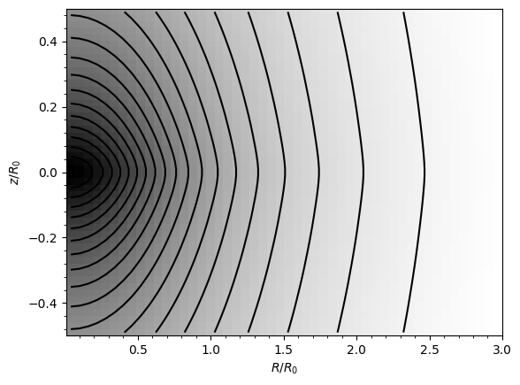
Plotting potentials

galpy potentials have built-in plotting methods:

# Plot the potential in the (R, z) plane
mp.plot(rmin=0.01, rmax=3.0, zmin=-0.5, zmax=0.5, nrs=50, nzs=50);

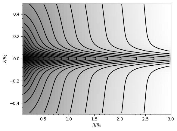
We can also plot the density of a composite potential like MWPotential2014:

# Plot the density
potential.plotDensities(
    MWPotential2014, rmin=0.1, rmax=3.0, zmin=-0.5, zmax=0.5, nrs=50, nzs=50, log=True
);

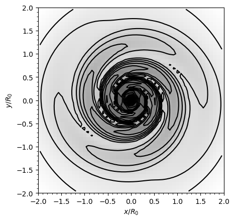
For non-axisymmetric potentials, we can plot the density in the x-y plane using xy=True:

from galpy.potential import SpiralArmsPotential

sp = SpiralArmsPotential(amp=0.6)
lp = LogarithmicHaloPotential(normalize=1.0)
potential.plotDensities(
    sp + lp, rmin=-2.0, rmax=2.0, zmin=-2.0, zmax=2.0, nrs=50, nzs=50, log=True, xy=True
)
plt.gca().set_aspect("equal");

Circular-orbit quantities

galpy can compute the circular velocity, epicycle frequency, vertical frequency, and angular frequency:

print("v_circ(R=1):", MWPotential2014.vcirc(1.0))
print("Omega_c(R=1):", MWPotential2014.omegac(1.0))
print("Epicycle freq(R=1):", MWPotential2014.epifreq(1.0))
print("Vertical freq(R=1):", MWPotential2014.verticalfreq(1.0))

v_circ(R=1): 1.0
Omega_c(R=1): 1.0
Epicycle freq(R=1): 1.340959647011537
Vertical freq(R=1): 2.7255405754769875

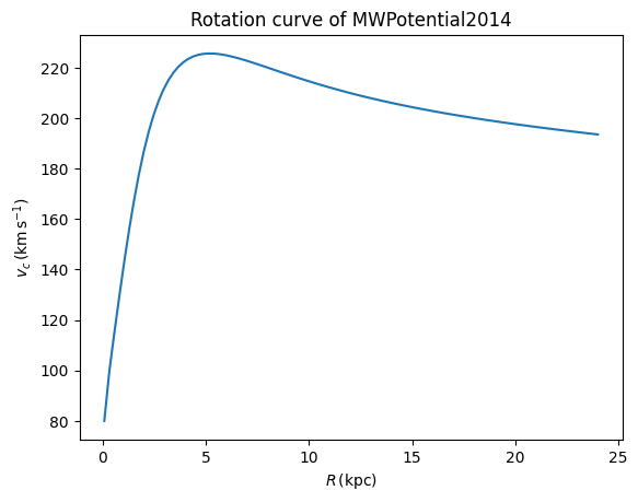
Let’s plot the rotation curve of MWPotential2014:

# Plot the rotation curve
Rs = numpy.linspace(0.01, 3.0, 101)
plt.plot(Rs * 8, [MWPotential2014.vcirc(R, ro=8.0, vo=220.0) for R in Rs])
plt.xlabel(r"$R\,(\mathrm{kpc})$")
plt.ylabel(r"$v_c\,(\mathrm{km\,s}^{-1})$")
plt.title("Rotation curve of MWPotential2014");

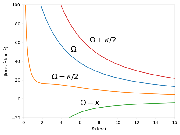
Spiral density wave diagram: \(\Omega - n\kappa/m\)

As an application of the above, we can compute the diagram of \(\Omega - n\kappa/m\), which is important for understanding kinematic spiral density waves. It shows the locations of various resonances.

def OmegaMinusKappa(pot, Rs, n, m, ro=8.0, vo=220.0):
    return pot.omegac(Rs / ro, ro=ro, vo=vo) - n / m * pot.epifreq(
        Rs / ro, ro=ro, vo=vo
    )


Rs = numpy.linspace(0.01, 16.0, 101)
plt.plot(Rs, OmegaMinusKappa(MWPotential2014, Rs, 0, 1))
plt.plot(Rs, OmegaMinusKappa(MWPotential2014, Rs, 1, 2))
plt.plot(Rs, OmegaMinusKappa(MWPotential2014, Rs, 1, 1))
plt.plot(Rs, OmegaMinusKappa(MWPotential2014, Rs, 1, -2))
plt.xlim(0.0, 16.0)
plt.ylim(-20.0, 100.0)
plt.xlabel(r"$R\,(\mathrm{kpc})$")
plt.ylabel(r"$(\mathrm{km\,s}^{-1}\,\mathrm{kpc}^{-1})$")
plt.text(3.0, 21.0, r"$\Omega-\kappa/2$", size=18.0)
plt.text(5.0, 50.0, r"$\Omega$", size=18.0)
plt.text(7.0, 60.0, r"$\Omega+\kappa/2$", size=18.0)
plt.text(6.0, -7.0, r"$\Omega-\kappa$", size=18.0);

Lindblad resonances

Find the radius of the inner and outer Lindblad resonances for a given pattern speed:

# Lindblad resonances for a pattern speed similar to the Milky Way's bar
# Using the Miyamoto-Nagai potential for this example:
print("Corotation:", mp.lindbladR(5.0 / 3.0, m="corotation"))
print("Inner Lindblad resonance (m=2):", mp.lindbladR(5.0 / 3.0, m=2))
print("Outer Lindblad resonance (m=-2):", mp.lindbladR(5.0 / 3.0, m=-2))

Corotation: 0.6027911166042229
Inner Lindblad resonance (m=2): None
Outer Lindblad resonance (m=-2): 0.9906190683480501

The None for m=2 means there is no inner Lindblad resonance for this potential.

Interpolated potentials

For expensive potentials, galpy provides interpRZPotential (for axisymmetric potentials) and interpSphericalPotential (for spherical potentials) that pre-compute a grid and interpolate. interpSphericalPotential can be initialized from a function giving the radial force or from an existing spherical potential. See the API documentation for full details.

from galpy.potential import interpRZPotential

# Create an interpolated version of MWPotential2014
ip = interpRZPotential(
    RZPot=MWPotential2014,
    rgrid=(0.01, 3.0, 51),
    zgrid=(0.0, 0.5, 26),
    interpPot=True,
    interpRforce=True,
    interpzforce=True,
)
# Compare
print("Original:", potential.evaluatePotentials(MWPotential2014, 1.0, 0.1))
print("Interpolated:", ip(1.0, 0.1))

Original: -1.3531320418152721
Interpolated: -1.3531320418152721

These interpolated potentials can be used anywhere a regular potential can be used, and they are much faster to evaluate than the original potential. They are especially useful for orbit integration, where the potential is evaluated many times.

Initializing potentials with physical parameters

You can initialize potentials directly with physical parameters (e.g., amp in \(M_\odot\), a in kpc) by passing ro= and vo=. When initialized this way, physical output is turned on automatically. Use use_physical=False to get output in natural units when needed.

from astropy import units as u

# NFW halo with physical parameters -- physical output is on by default
nfw = NFWPotential(mvir=1.0, conc=15.0, ro=8.0, vo=220.0)

# Output is in physical units (km^2/s^2) automatically
print("Phi(R=1, z=0) [physical]:", nfw(1.0, 0.0), "km^2/s^2")

# Use use_physical=False to get natural units
print("Phi(R=1, z=0) [natural]:", nfw(1.0, 0.0, use_physical=False))

# You can also pass astropy Quantities directly
print("Phi(8 kpc, 0 kpc):", nfw(8.0 * u.kpc, 0.0 * u.kpc), "km^2/s^2")

Phi(R=1, z=0) [physical]: -96354.67477240822 km^2/s^2
Phi(R=1, z=0) [natural]: -1.9907990655456245
Phi(8 kpc, 0 kpc): -96354.67477240822 km^2/s^2

This also works for other potential types, such as MiyamotoNagaiPotential:

# Miyamoto-Nagai with physical amplitude (amp in Msun, a and b in kpc)
mn_phys = MiyamotoNagaiPotential(
    amp=5e10 * u.Msun, a=3.0 * u.kpc, b=0.28 * u.kpc, ro=8.0, vo=220.0
)
print("v_circ(R=1) [physical]:", mn_phys.vcirc(1.0), "km/s")
print("v_circ(R=1) [natural]:", mn_phys.vcirc(1.0, use_physical=False))

# turn_physical_off / turn_physical_on lets you switch the default
mn_phys.turn_physical_off()
print("\nAfter turn_physical_off:")
print("v_circ(R=1):", mn_phys.vcirc(1.0))

mn_phys.turn_physical_on(ro=8.0, vo=220.0)
print("\nAfter turn_physical_on:")
print("v_circ(R=1):", mn_phys.vcirc(1.0), "km/s")

v_circ(R=1) [physical]: 145.9185599862874 km/s
v_circ(R=1) [natural]: 0.6632661817558517

After turn_physical_off:
v_circ(R=1): 0.6632661817558517

After turn_physical_on:
v_circ(R=1): 145.9185599862874 km/s

Tip

The amp= parameter has different units for different potentials. Check each potential’s documentation to learn what the units are. For example, for a LogarithmicHaloPotential the units are velocity squared, while for a MiyamotoNagaiPotential they are units of mass. Check each potential’s API documentation for the units of amp=.

Warning

When combining potentials with different ro= and vo= values, unexpected behavior can result. It is best to use the same ro= and vo= for all potentials in a combination.