This page was generated from a Jupyter notebook. You can download it here.

Multiple Orbits

galpy’s Orbit class natively handles multiple orbits at once, enabling efficient parallel integration and vectorized access to orbital quantities.

For basic orbit initialization, see Orbit Initialization.

%matplotlib inline
import numpy
from astropy import units
from astropy.coordinates import SkyCoord
from galpy.orbit import Orbit
from galpy.potential import MWPotential2014
import warnings

warnings.filterwarnings("ignore", category=RuntimeWarning)
warnings.filterwarnings("ignore", category=UserWarning)

Array initialization

Pass a 2D array of shape (N, dim) to create N orbits at once.

numpy.random.seed(42)
N = 10
vxvvs = numpy.column_stack(
    [
        numpy.random.uniform(0.8, 1.2, N),  # R
        numpy.random.normal(0.0, 0.05, N),  # vR
        numpy.random.uniform(0.9, 1.1, N),  # vT
        numpy.random.normal(0.0, 0.05, N),  # z
        numpy.random.normal(0.0, 0.05, N),  # vz
        numpy.random.uniform(0.0, 2 * numpy.pi, N),  # phi
    ]
)
os = Orbit(vxvvs)
print("Number of orbits:", os.size)
print("Shape:", os.shape)
print("R values:", os.R())

Number of orbits: 10
Shape: (10,)
R values: [0.94981605 1.18028572 1.09279758 1.03946339 0.86240746 0.86239781
 0.82323344 1.14647046 1.040446   1.08322903]

Orbits can have arbitrary shapes that are preserved for all outputs. For example, to create a 2D grid of orbits, we can do:

numpy.random.seed(42)
N, M = 10, 5
vxvvs_2d = numpy.stack(
    [
        numpy.random.uniform(0.8, 1.2, size=(N, M)),  # R
        numpy.random.normal(0.0, 0.05, size=(N, M)),  # vR
        numpy.random.uniform(0.9, 1.1, size=(N, M)),  # vT
        numpy.random.normal(0.0, 0.05, size=(N, M)),  # z
        numpy.random.normal(0.0, 0.05, size=(N, M)),  # vz
        numpy.random.uniform(0.0, 2 * numpy.pi, size=(N, M)),  # phi
    ],
    axis=-1,
)
os = Orbit(vxvvs_2d)
print("Number of orbits:", os.size)
print("Shape:", os.shape)
print("R values:", os.R())

Number of orbits: 50
Shape: (10, 5)
R values: [[0.94981605 1.18028572 1.09279758 1.03946339 0.86240746]
 [0.86239781 0.82323344 1.14647046 1.040446   1.08322903]
 [0.8082338  1.18796394 1.13297706 0.88493564 0.87272999]
 [0.8733618  0.9216969  1.00990257 0.97277801 0.91649166]
 [1.04474116 0.85579754 0.91685786 0.94654474 0.98242799]
 [1.11407038 0.87986951 1.00569378 1.03696583 0.81858017]
 [1.04301794 0.86820965 0.82602064 1.17955421 1.18625281]
 [1.12335894 0.92184551 0.83906885 1.07369321 0.976061  ]
 [0.84881529 0.99807076 0.81375541 1.16372816 0.90351199]
 [1.06500891 0.92468443 1.00802721 1.01868411 0.87394178]]

Initialization from SkyCoord arrays

You can pass a SkyCoord containing multiple objects.

sc = SkyCoord(
    ra=[20.0, 50.0, 100.0] * units.deg,
    dec=[30.0, -10.0, 45.0] * units.deg,
    distance=[1.5, 3.0, 0.8] * units.kpc,
    pm_ra_cosdec=[3.5, -1.0, 2.0] * units.mas / units.yr,
    pm_dec=[-1.2, 0.5, -0.3] * units.mas / units.yr,
    radial_velocity=[15.0, -30.0, 50.0] * units.km / units.s,
)
os_sc = Orbit(sc)
print("Number of orbits:", os_sc.size)
print("RA values:", os_sc.ra())

galpyWarning: Supplied SkyCoord does not contain (galcen_distance, z_sun, galcen_v_sun) and these were not explicitly set in the Orbit initialization using the keywords (ro, zo, vo, solarmotion); these are required for Orbit initialization; proceeding with default values
Number of orbits: 3
RA values: [ 20.  50. 100.]

List initialization

A list of phase-space arrays also works.

os_list = Orbit(
    [
        [1.0, 0.1, 1.0, 0.0, 0.05, 0.0],
        [0.9, -0.05, 1.1, 0.02, -0.03, 1.0],
    ]
)
print("Size:", os_list.size)
print("R:", os_list.R())

Size: 2
R: [1.  0.9]

or a list or Orbit instances, e.g.:

os_list = Orbit(
    [
        Orbit([1.0, 0.1, 1.0, 0.0, 0.05, 0.0]),
        Orbit([0.9, -0.05, 1.1, 0.02, -0.03, 1.0]),
    ]
)
print("Size:", os_list.size)
print("R:", os_list.R())

Size: 2
R: [1.  0.9]

Shape, len, size, and reshape

Multi-orbit objects behave like arrays.

os_many = Orbit(vxvvs)
print("len:", len(os_many))
print("size:", os_many.size)
print("shape:", os_many.shape)

# Reshape to (2, 5) -- reshape is done in-place
os_many.reshape((2, 5))
print("Reshaped shape:", os_many.shape)
print("Reshaped len:", len(os_many))

len: 10
size: 10
shape: (10,)
Reshaped shape: (2, 5)
Reshaped len: 2

Slicing and indexing

Indexing and slicing returns a new Orbit object.

# Single orbit (from the flat os object)
os_flat = Orbit(vxvvs)
o_single = os_flat[3]
print("Single orbit:", o_single)
print("Size:", o_single.size)

# Slice
o_slice = os_flat[2:5]
print("Slice size:", o_slice.size)

# 2D indexing on reshaped
o_2d = os_many[1, 2]
print("2D indexed orbit R:", o_2d.R())

Single orbit: <galpy.orbit.Orbits.Orbit object at 0x7f0b9bdbb050>
Size: 1
Slice size: 3
2D indexed orbit R: 1.146470458309974

Output shapes are preserved

When you access quantities from a multi-orbit object, the output has the same shape as the orbit array.

print("R shape (flat):", os_flat.R().shape)
print("R shape (reshaped):", os_many.R().shape)

R shape (flat): (10,)
R shape (reshaped): (2, 5)

Array-valued Solar parameters

You can pass arrays for ro, zo, and vo, as well as an array-valued solarmotion, when initializing multiple orbits from observed coordinates. This is useful when propagating uncertainty in Solar parameters across many orbit realizations.

The scalar-parameter arrays should have the same shape as the orbit array. For a one-dimensional orbit array of length N, solarmotion should have shape (3, N).

lb_data = numpy.tile([20.0, 30.0, 2.0, -10.0, 20.0, 50.0], (3, 1))
solarmotion = numpy.array(
    [
        [10.0, 11.0, 12.0],
        [11.0, 12.0, 13.0],
        [7.0, 7.5, 8.0],
    ]
)
os_phys = Orbit(
    lb_data,
    lb=True,
    ro=numpy.array([8.0, 8.2, 8.4]),
    zo=numpy.array([0.015, 0.0208, 0.03]),
    vo=numpy.array([220.0, 225.0, 230.0]),
    solarmotion=solarmotion,
)
print("R (physical):", os_phys.R())
print("z (physical):", os_phys.z())
print("vR (physical):", os_phys.vR())

R (physical): [6.39801729 6.5965276  6.79471746]
z (physical): [1.01194971 1.01667146 1.02418402]
vR (physical): [37.01873757 38.08904318 39.07811118]

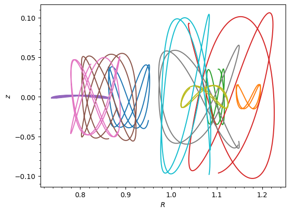
Integrating and plotting multiple orbits

When integrating multiple orbits, output array have an additional T dimension with T the number of time steps. This allows you to easily access the integrated trajectories of all orbits.

When plotting multiple orbits, each orbit is plotted with a different color by default.

from matplotlib import pyplot as plt

# Integrate all 10 orbits and plot them
os_plot = Orbit(vxvvs)
ts = numpy.linspace(0.0, 10.0, 1001)
os_plot.integrate(ts, MWPotential2014)
print("Integrated shape:", os_plot.R(ts).shape)
os_plot.plot();

Integrated shape: (10, 1001)

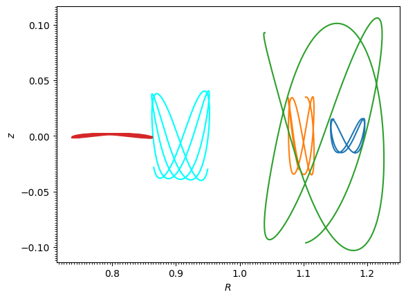
When slicing or indexing a multi-orbit object, the resulting single orbit object retains the integrated trajectory of the original multi-orbit object, so you can still plot it without re-integrating:

print(f"Shape of os_plot[1].R(ts): {os_plot[1].R(ts).shape}")
print(f"Shape of os_plot[3:9].R(ts): {os_plot[3:9].R(ts).shape}")
os_plot[0].plot(color="cyan")  # Plot the first orbit in a different color
os_plot[1:5].plot(overplot=True)  # Plot orbits 1-4 in default colors
plt.gca().autoscale();

Shape of os_plot[1].R(ts): (1001,)
Shape of os_plot[3:9].R(ts): (6, 1001)

Per-orbit integration time arrays

By default, Orbit.integrate(t, pot) uses a single shared time array t for every orbit in the instance. You can also pass per-orbit time arrays by giving t a shape that matches the Orbit shape with an additional time axis at the end — i.e. (*orbit.shape, nt). Each orbit is then integrated on its own time grid, while still benefiting from the batched, multi-threaded C integrator.

This is useful when each orbit has a natural integration window of its own, e.g. tail particles in a tidal stream, each integrated from its individual stripping time to the present.

Note that orbit-continuation (re-integrating to extend an already-integrated orbit) is not supported in this mode — each call to integrate with a per-orbit t restarts from the original initial conditions.

os_indiv = Orbit(vxvvs)  # 10 orbits
# Each orbit gets its own time grid; here from 0 to t_end[i]
t_end = numpy.linspace(5.0, 12.0, os_indiv.size)
ts_indiv = numpy.linspace(
    numpy.zeros(os_indiv.size), t_end, 1001, axis=-1
)  # shape (10, 1001)
os_indiv.integrate(ts_indiv, MWPotential2014, method="dop853_c")
print("orbit storage shape:", os_indiv.orbit.shape)
print("per-orbit time-array shape:", os_indiv.t.shape)

orbit storage shape: (10, 1001, 6)
per-orbit time-array shape: (10, 1001)