Two-dimensional disk distribution functions
galpy contains various disk distribution functions, both in two and three dimensions. This section introduces the two-dimensional distribution functions, useful for studying the dynamics of stars that stay relatively close to the mid-plane of a galaxy. The vertical motions of these stars may be approximated as being entirely decoupled from the motion in the plane.
Types of disk distribution functions
galpy contains the following distribution functions for razor-thin
disks: galpy.df.dehnendf, galpy.df.shudf, and
galpy.df.schwarzschilddf. These are the distribution functions of
Dehnen (1999AJ….118.1201D), Shu
(1969ApJ…158..505S), and
Schwarzschild (the Shu DF in the epicycle approximation, see Binney &
Tremaine 2008). Everything shown below for dehnendf can also be
done for shudf and schwarzschilddf. The Schwarzschild DF is
primarily included as an educational tool; it is not a true
steady-state DF, because it uses the approximate energy from the
epicycle approximation rather than the true energy, and is fully
superseded by the Shu DF, which is a good steady-state DF.
These disk distribution functions are functions of the energy and the
angular momentum alone. They can be evaluated for orbits, or for a
given energy and angular momentum. At this point, only power-law
rotation curves are supported. A dehnendf instance is initialized
as follows
>>> from galpy.df import dehnendf
>>> dfc= dehnendf(beta=0.)
This initializes a dehnendf instance based on an exponential
surface-mass profile with scale-length 1/3 and an exponential
radial-velocity-dispersion profile with scale-length 1 and a value of
0.2 at R=1. Different parameters for these profiles can be provided as
an initialization keyword. For example,
>>> dfc= dehnendf(beta=0.,profileParams=(1./4.,1.,0.2))
initializes the distribution function with a radial scale length of 1/4 instead.
We can show that these distribution functions have an asymmetric drift built-in by evaluating the DF at R=1. We first create a set of orbit-instances and then evaluate the DF at them
>>> from galpy.orbit import Orbit
>>> os= [Orbit([1.,0.,1.+-0.9+1.8/1000*ii]) for ii in range(1001)]
>>> dfro= [dfc(o) for o in os]
>>> plot([1.+-0.9+1.8/1000*ii for ii in range(1001)],dfro)
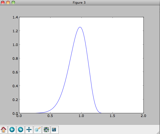
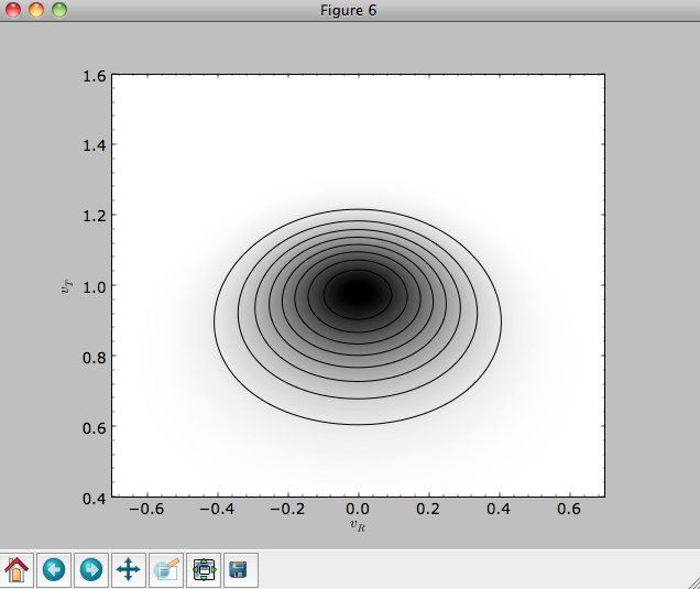
Or we can plot the two-dimensional density at R=1.
>>> dfro= [[dfc(Orbit([1.,-0.7+1.4/200*jj,1.-0.6+1.2/200*ii])) for jj in range(201)]for ii in range(201)]
>>> dfro= numpy.array(dfro)
>>> from galpy.util.plot import dens2d
>>> dens2d(dfro,origin='lower',cmap='gist_yarg',contours=True,xrange=[-0.7,0.7],yrange=[0.4,1.6],xlabel=r'$v_R$',ylabel=r'$v_T$')
Evaluating moments of the DF
galpy can evaluate various moments of the disk distribution functions. For example, we can calculate the mean velocities (for the DF with a scale length of 1/3 above)
>>> dfc.meanvT(1.)
# 0.91715276979447324
>>> dfc.meanvR(1.)
# 0.0
and the velocity dispersions
>>> numpy.sqrt(dfc.sigmaR2(1.))
# 0.19321086259083936
>>> numpy.sqrt(dfc.sigmaT2(1.))
# 0.15084122011271159
and their ratio
>>> dfc.sigmaR2(1.)/dfc.sigmaT2(1.)
# 1.6406766813028968
In the limit of zero velocity dispersion (the epicycle approximation) this ratio should be equal to 2, which we can check as follows
>>> dfccold= dehnendf(beta=0.,profileParams=(1./3.,1.,0.02))
>>> dfccold.sigmaR2(1.)/dfccold.sigmaT2(1.)
# 1.9947493895454664
We can also calculate higher order moments
>>> dfc.skewvT(1.)
# -0.48617143862047763
>>> dfc.kurtosisvT(1.)
# 0.13338978593181494
>>> dfc.kurtosisvR(1.)
# -0.12159407676394096
We already saw above that the velocity dispersion at R=1 is not
exactly equal to the input velocity dispersion (0.19321086259083936
vs. 0.2). Similarly, the whole surface-density and velocity-dispersion
profiles are not quite equal to the exponential input profiles. We can
calculate the resulting surface-mass density profile using
surfacemass, sigmaR2, and sigma2surfacemass. The latter
calculates the product of the velocity dispersion squared and the
surface-mass density. E.g.,
>>> dfc.surfacemass(1.)
# 0.050820867101511534
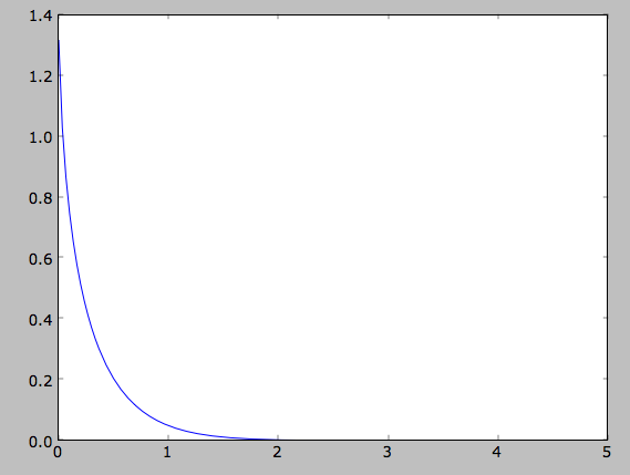
We can plot the surface-mass density as follows
>>> Rs= numpy.linspace(0.01,5.,151)
>>> out= [dfc.surfacemass(r) for r in Rs]
>>> plot(Rs, out)
or
>>> plot(Rs,numpy.log(out))
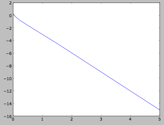
which shows the exponential behavior expected for an exponential disk. We can compare this to the input surface-mass density
>>> input_out= [dfc.targetSurfacemass(r) for r in Rs]
>>> plot(Rs,numpy.log(input_out)-numpy.log(out))
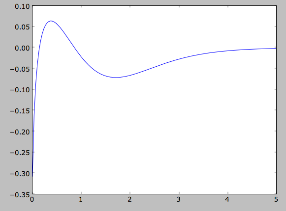
which shows that there are significant differences between the desired surface-mass density and the actual surface-mass density. We can do the same for the velocity-dispersion profile
>>> out= [dfc.sigmaR2(r) for r in Rs]
>>> input_out= [dfc.targetSigma2(r) for r in Rs]
>>> plot(Rs,numpy.log(input_out)-numpy.log(out))
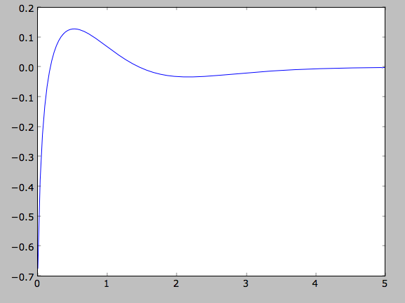
That the input surface-density and velocity-dispersion profiles are not the same as the output profiles, means that estimates of DF properties based on these profiles will not be quite correct. Obviously this is the case for the surface-density and velocity-dispersion profiles themselves, which have to be explicitly calculated by integration over the DF rather than by evaluating the input profiles. This also means that estimates of the asymmetric drift based on the input profiles will be wrong. We can calculate the asymmetric drift at R=1 using the asymmetric drift equation derived from the Jeans equation (eq. 4.228 in Binney & Tremaine 2008), using the input surface-density and velocity dispersion profiles
>>> dfc.asymmetricdrift(1.)
# 0.090000000000000024
which should be equal to the circular velocity minus the mean rotational velocity
>>> 1.-dfc.meanvT(1.)
# 0.082847230205526756
These are not the same in part because of the difference between the
input and output surface-density and velocity-dispersion profiles (and
because the asymmetricdrift method assumes that the ratio of the
velocity dispersions squared is two using the epicycle approximation;
see above).
Using corrected disk distribution functions
As shown above, for a given surface-mass density and velocity
dispersion profile, the two-dimensional disk distribution functions
only do a poor job of reproducing the desired profiles. We can correct
this by calculating a set of corrections to the input profiles such
that the output profiles more closely resemble the desired profiles
(see 1999AJ….118.1201D). galpy supports
the calculation of these corrections, and comes with some
pre-calculated corrections bundled with the code. For
example, the following initializes a dehnendf with corrections up
to 20th order (the default)
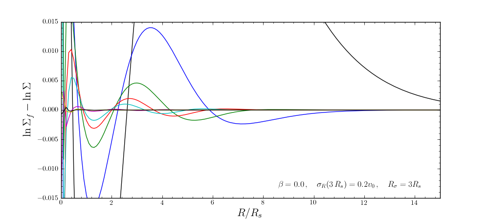
>>> dfc= dehnendf(beta=0.,correct=True)
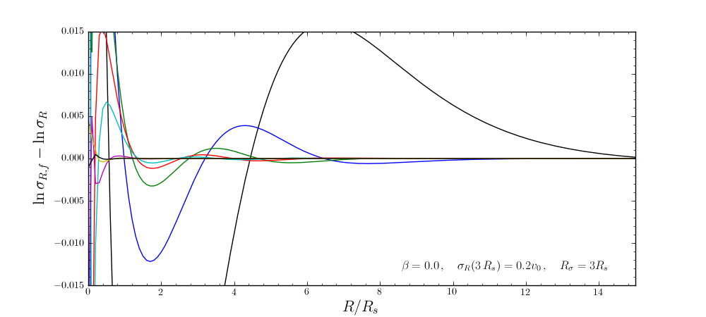
The following figure shows the difference between the actual surface-mass density profile and the desired profile for 1, 2, 3, 4, 5, 10, 15, and 20 iterations
and the same for the velocity-dispersion profile
galpy will automatically save any new corrections that you calculate.
All of the methods for an uncorrected disk DF can be used for the corrected DFs as well. For example, the velocity dispersion is now
>>> numpy.sqrt(dfc.sigmaR2(1.))
# 0.19999985069451526
and the mean rotation velocity is
>>> dfc.meanvT(1.)
# 0.90355161181498711
and (correct) asymmetric drift
>>> 1.-dfc.meanvT(1.)
# 0.09644838818501289
That this still does not agree with the simple dfc.asymmetricdrift
estimate is because of the latter’s using the epicycle approximation
for the ratio of the velocity dispersions.
Oort constants and functions
galpy also contains methods to calculate the Oort functions for two-dimensional disk distribution functions. These are known as the Oort constants when measured in the solar neighborhood. They are combinations of the mean velocities and derivatives thereof. galpy calculates these by direct integration over the DF and derivatives of the DF. Thus, we can calculate
>>> dfc= dehnendf(beta=0.)
>>> dfc.oortA(1.)
# 0.43190780889218749
>>> dfc.oortB(1.)
# -0.48524496090228575
The K and C Oort constants are zero for axisymmetric DFs
>>> dfc.oortC(1.)
# 0.0
>>> dfc.oortK(1.)
# 0.0
In the epicycle approximation, for a flat rotation curve A =- B = 0.5. The explicit calculates of A and B for warm DFs quantify how good (or bad) this approximation is
>>> dfc.oortA(1.)+dfc.oortB(1.)
# -0.053337152010098254
For the cold DF from above the approximation is much better
>>> dfccold= dehnendf(beta=0.,profileParams=(1./3.,1.,0.02))
>>> dfccold.oortA(1.), dfccold.oortB(1.)
# (0.49917556666144003, -0.49992824742490816)
Sampling data from the DF
We can sample from the disk distribution functions using
sample. sample can return either an energy–angular-momentum
pair, or a full orbit initialization. We can sample 4000 orbits for
example as (could take two minutes)
>>> o= dfc.sample(n=4000,returnOrbit=True,nphi=1)
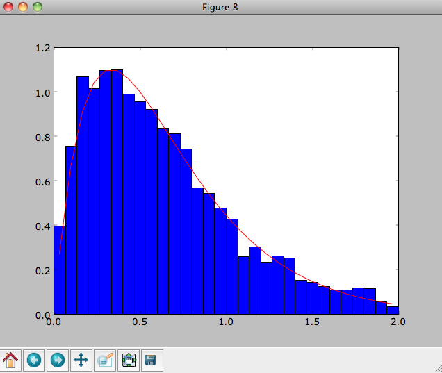
We can then plot the histogram of the sampled radii and compare it to the input surface-mass density profile
>>> Rs= [e.R() for e in o]
>>> hists, bins, edges= hist(Rs,range=[0,2],normed=True,bins=30)
>>> xs= numpy.array([(bins[ii+1]+bins[ii])/2. for ii in range(len(bins)-1)])
>>> plot(xs, xs*exp(-xs*3.)*9.,'r-')
E.g.,
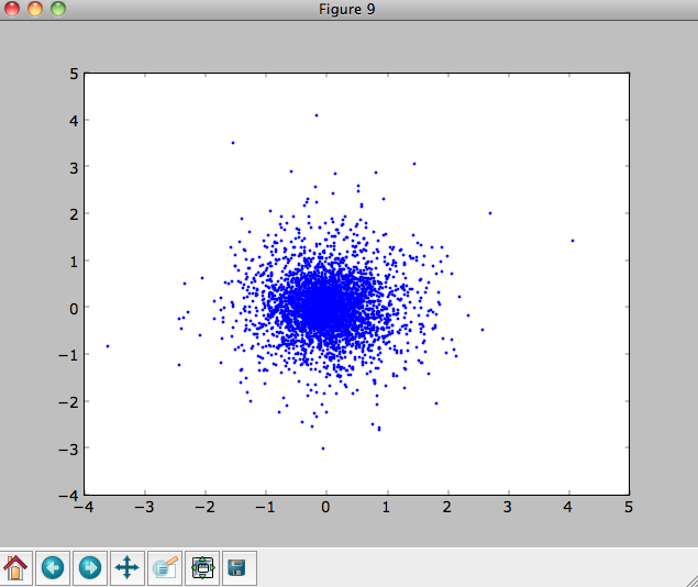
We can also plot the spatial distribution of the sampled disk
>>> xs= [e.x() for e in o]
>>> ys= [e.y() for e in o]
>>> figure()
>>> plot(xs,ys,',')
E.g.,
We can also sample points in a specific radial range (might take a few minutes)
>>> o= dfc.sample(n=1000,returnOrbit=True,nphi=1,rrange=[0.8,1.2])
and we can plot the distribution of rotational velocities
>>> vTs= [e.vxvv[2] for e in o]
>>> hists, bins, edges= hist(vTs,range=[.5,1.5],normed=True,bins=30)
>>> xs= numpy.array([(bins[ii+1]+bins[ii])/2. for ii in range(len(bins)-1)])
>>> dfro= [dfc(Orbit([1.,0.,x]))/9./numpy.exp(-3.) for x in xs]
>>> plot(xs,dfro,'r-')
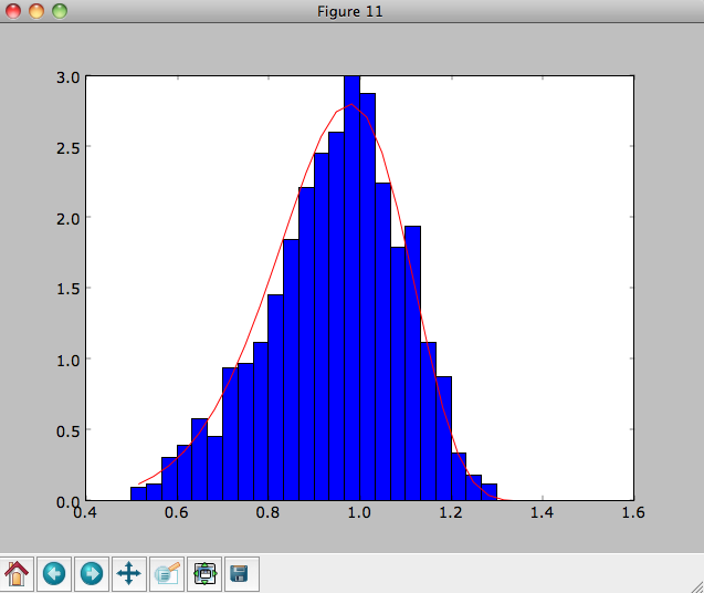
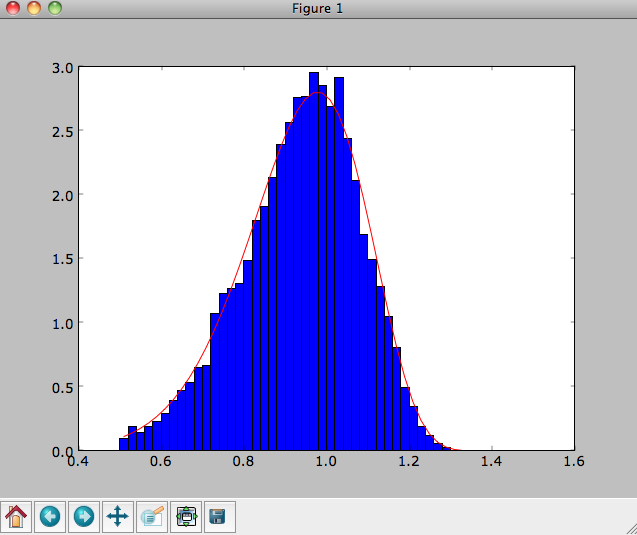
The agreement between the sampled distribution and the theoretical
curve is not as good because the sampled distribution has a finite
radial range. If we sample 10,000 points in rrange=[0.95,1.05] the
agreement is better (this takes a long time):
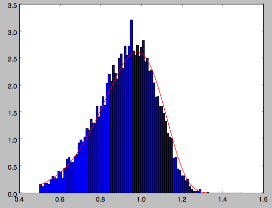
We can also directly sample velocities at a given radius rather than in a range of radii. Doing this for a correct DF gives
>>> dfc= dehnendf(beta=0.,correct=True)
>>> vrvt= dfc.sampleVRVT(1.,n=10000)
>>> hists, bins, edges= hist(vrvt[:,1],range=[.5,1.5],normed=True,bins=101)
>>> xs= numpy.array([(bins[ii+1]+bins[ii])/2. for ii in range(len(bins)-1)])
>>> dfro= [dfc(Orbit([1.,0.,x])) for x in xs]
>>> plot(xs,dfro/numpy.sum(dfro)/(xs[1]-xs[0]),'r-')
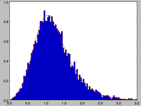
galpy further has support for sampling along a given line of sight in the disk, which is useful for interpreting surveys consisting of a finite number of pointings. For example, we can sampled distances along a given line of sight
>>> ds= dfc.sampledSurfacemassLOS(30./180.*numpy.pi,n=10000)
which is very fast. We can histogram these
>>> hists, bins, edges= hist(ds,range=[0.,3.5],normed=True,bins=101)
and compare it to the predicted distribution, which we can calculate as
>>> xs= numpy.array([(bins[ii+1]+bins[ii])/2. for ii in range(len(bins)-1)])
>>> fd= numpy.array([dfc.surfacemassLOS(d,30.) for d in xs])
>>> plot(xs,fd/numpy.sum(fd)/(xs[1]-xs[0]),'r-')
which shows very good agreement with the sampled distances
galpy can further sample full 4D phase–space coordinates along a
given line of sight through dfc.sampleLOS.
Non-axisymmetric, time-dependent disk distribution functions
galpy also supports the evaluation of non-axisymmetric,
time-dependent two-dimensional DFs. These specific DFs are constructed
by assuming an initial axisymmetric steady state, described by a DF of
the family discussed above, that is then acted upon by a
non-axisymmetric, time-dependent perturbation. The DF at a given time
and phase-space position is evaluated by integrating the orbit
backwards in time in the non-axisymmetric potential until the time of
the initial DF is reached. From Liouville’s theorem, which states that
phase-space volume is conserved along the orbit, we then know that we
can evaluate the non-axisymmetric DF today as the initial DF at the
initial point on the orbit. This procedure was first used by Dehnen
(2000).
This is implemented in galpy as galpy.df.evolveddiskdf. Such a
DF is setup by specifying the initial DF, the non-axisymmetric
potential, and the time of the initial state. For example, we can look
at the effect of an elliptical perturbation to the potential like that
described by Kuijken & Tremaine. To do this, we
set up an elliptical perturbation to a logarithmic potential that is
grown slowly to minimize non-adiabatic effects
>>> from galpy.potential import LogarithmicHaloPotential, EllipticalDiskPotential
>>> lp= LogarithmicHaloPotential(normalize=1.)
>>> ep= EllipticalDiskPotential(twophio=0.05,phib=0.,p=0.,tform=-150.,tsteady=125.)
This perturbation starts to be grown at tform=-150 over a time
period of tsteady=125 time units. We will consider the effect of
this perturbation on a very cold disk (velocity dispersion
\(\sigma_R = 0.0125\,v_c\)) and a warm disk (\(\sigma_R =
0.15\,v_c\)). We set up these two initial DFs
>>> idfcold= dehnendf(beta=0.,profileParams=(1./3.,1.,0.0125))
>>> idfwarm= dehnendf(beta=0.,profileParams=(1./3.,1.,0.15))
and then set up the evolveddiskdf
>>> from galpy.df import evolveddiskdf
>>> edfcold= evolveddiskdf(idfcold,[lp,ep],to=-150.)
>>> edfwarm= evolveddiskdf(idfwarm,[lp,ep],to=-150.)
where we specify that the initial state is at to=-150.
We can now use these evolveddiskdf instances in much the same way
as diskdf instances. One difference is that there is much more
support for evaluating the DF on a grid (to help speed up the rather
slow computations involved). Thus, we can evaluate the mean radial
velocity at R=0.9, phi=22.5 degree, and t=0 by using a grid
>>> mvrcold, gridcold= edfcold.meanvR(0.9,phi=22.5,deg=True,t=0.,grid=True,returnGrid=True,gridpoints=51,nsigma=6.)
>>> mvrwarm, gridwarm= edfwarm.meanvR(0.9,phi=22.5,deg=True,t=0.,grid=True,returnGrid=True,gridpoints=51)
>>> print(mvrcold, mvrwarm)
# -0.0358753028951 -0.0294763627935
The cold response agrees well with the analytical calculation, which predicts that this is \(-0.05/\sqrt{2}\):
>>> print(mvrcold+0.05/sqrt(2.))
# -0.000519963835811
The warm response is slightly smaller in amplitude
>>> print(mvrwarm/mvrcold)
# 0.821633837619
although the numerical uncertainty in mvrwarm is large, because
the grid is not sufficiently fine.
We can then reuse this grid in calculations of other moments of the DF, e.g.,
>>> print(edfcold.meanvT(0.9,phi=22.5,deg=True,t=0.,grid=gridcold))
# 0.965058551359
>>> print(edfwarm.meanvT(0.9,phi=22.5,deg=True,t=0.,grid=gridwarm))
# 0.915397094614
which returns the mean rotational velocity, and
>>> print(edfcold.vertexdev(0.9,phi=22.5,deg=True,t=0.,grid=gridcold))
# 0.0560531474616
>>> print(edfwarm.vertexdev(0.9,phi=22.5,deg=True,t=0.,grid=gridwarm))
# 0.0739164830253
which gives the vertex deviation in rad. The reason we have to
calculate the grid out to 6nsigma for the cold response is that
the response is much bigger than the velocity dispersion of the
population. This velocity dispersion is used to automatically to set
the grid edges, but sometimes has to be adjusted to contain the full
DF.
evolveddiskdf can also calculate the Oort functions, by directly
calculating the spatial derivatives of the DF. These can also be calculated on a grid, such that we can do
>>> oortacold, gridcold, gridrcold, gridphicold= edfcold.oortA(0.9,phi=22.5,deg=True,t=0.,returnGrids=True,gridpoints=51,derivGridpoints=51,grid=True,derivphiGrid=True,derivRGrid=True,nsigma=6.)
>>> oortawarm, gridwarm, gridrwarm, gridphiwarm= edfwarm.oortA(0.9,phi=22.5,deg=True,t=0.,returnGrids=True,gridpoints=51,derivGridpoints=51,grid=True,derivphiGrid=True,derivRGrid=True)
>>> print(oortacold, oortawarm)
# 0.575494559999 0.526389833249
It is clear that these are quite different. The cold calculation is again close to the analytical prediction, which says that \(A = A_{\mathrm{axi}}+0.05/(2\sqrt{2})\) where \(A_{\mathrm{axi}} = 1/(2\times0.9)\) in this case:
>>> print(oortacold-(0.5/0.9+0.05/2./sqrt(2.)))
# 0.0022613349141670236
These grids can then be reused for the other Oort functions, for example,
>>> print(edfcold.oortB(0.9,phi=22.5,deg=True,t=0.,grid=gridcold,derivphiGrid=gridphicold,derivRGrid=gridrcold))
# -0.574674310521
>>> print(edfwarm.oortB(0.9,phi=22.5,deg=True,t=0.,grid=gridwarm,derivphiGrid=gridphiwarm,derivRGrid=gridrwarm))
# -0.555546911144
and similar for oortC and oortK. These warm results should
again be considered for illustration only, as the grid is not
sufficiently fine to have a small numerical error.
The grids that have been calculated can also be plotted to show the full velocity DF. For example,
>>> gridcold.plot()
gives
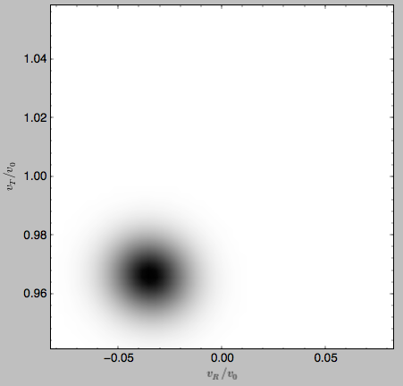
which demonstrates that the DF is basically the initial DF that has been displaced (by a significant amount compared to the velocity dispersion). The warm velocityd distribution is given by
>>> gridwarm.plot()
which returns
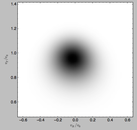
The shift of the smooth DF here is much smaller than the velocity dispersion.
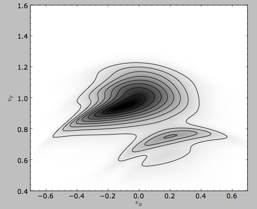
Example: The Hercules stream in the Solar neighborhood as a result of the Galactic bar
We can combine the orbit integration capabilities of galpy with the provided distribution functions and see the effect of the Galactic bar on stellar velocities. By backward integrating orbits starting at the Solar position in a potential that includes the Galactic bar we can evaluate what the velocity distribution is that we should see today if the Galactic bar stirred up a steady-state disk. For this we initialize a flat rotation curve potential and Dehnen’s bar potential
>>> from galpy.potential import LogarithmicHaloPotential, DehnenBarPotential
>>> lp= LogarithmicHaloPotential(normalize=1.)
>>> dp= DehnenBarPotential()
The Dehnen bar potential is initialized to start bar formation four bar periods before the present day and to have completely formed the bar two bar periods ago. We can integrate back to the time before bar-formation:
>>> ts= numpy.linspace(0,dp.tform(),1000)
where dp.tform() is the time of bar-formation (in the usual
time-coordinates).
We initialize orbits on a grid in velocity space and integrate them
>>> ins= Orbit(numpy.array([[[1.,-0.7+1.4/100*jj,1.-0.6+1.2/100*ii,0.] for jj in range(101)] for ii in range(101)]))
>>> ins.integrate(ts,[lp,dp])
We can then evaluate the weight of these orbits by assuming that the
disk was in a steady-state before bar-formation with a Dehnen
distribution function. We evaluate the Dehnen distribution function at
dp.tform() for each of the orbits (evaluating the distribution
function only works for an Orbit with a single object, so we need to
unpack the Orbit instance that contains all orbits)
>>> dfc= dehnendf(beta=0.,correct=True)
>>> out= [[dfc(o(dp.tform())) for o in j] for j in ins]
>>> out= numpy.array(out)
This gives
>>> from galpy.util.plot import dens2d
>>> dens2d(out,origin='lower',cmap='gist_yarg',contours=True,xrange=[-0.7,0.7],yrange=[0.4,1.6],xlabel=r'$v_R$',ylabel=r'$v_T$')
Now that galpy contains the evolveddiskdf described above,
this whole calculation is encapsulated in this module and can be done
much more easily as
>>> edf= evolveddiskdf(dfc,[lp,dp],to=dp.tform())
>>> mvr, grid= edf.meanvR(1.,grid=True,gridpoints=101,returnGrid=True)
The gridded DF can be accessed as grid.df, which we can plot as before
>>> dens2d(grid.df.T,origin='lower',cmap='gist_yarg',contours=True,xrange=[grid.vRgrid[0],grid.vRgrid[-1]],yrange=[grid.vTgrid[0],grid.vTgrid[-1]],xlabel=r'$v_R$',ylabel=r'$v_T$')
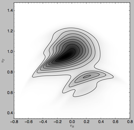
For more information see 2000AJ….119..800D and 2010ApJ…725.1676B. Note that the x-axis in the Figure above is defined as minus the x-axis in these papers.
