Dynamical modeling of tidal streams

galpy contains tools to model the dynamics of tidal streams, making extensive use of action-angle variables and also containing a simple particle-spray method. Both of these are introduced in the following sections.

Modeling streams in action-angle coordinates with streamdf

Action-angle coordinates are ideal for modeling tidal streams in potentials that allow for the calculation of action-angle coordinates (any static potential in the absence of chaos, which describes at least regions such as the inner Milky-Way halo well). As an example of modeling streams in action-angle coordinates, we can investigate the dynamics of the following tidal stream (that of Bovy 2014; 2014ApJ…795…95B). This movie shows the disruption of a cluster on a GD-1-like orbit around the Milky Way:

The blue line is the orbit of the progenitor cluster and the black points are cluster members. The disruption is shown in an approximate orbital plane and the movie is comoving with the progenitor cluster.

Streams can be represented by simple dynamical models in action-angle coordinates. In action-angle coordinates, stream members are stripped from the progenitor cluster onto orbits specified by a set of actions \((J_R,J_\phi,J_Z)\), which remain constant after the stars have been stripped. This is shown in the following movie, which shows the generation of the stream in action space

The color-coding gives the angular momentum \(J_\phi\) and the black dot shows the progenitor orbit. These actions were calculated using galpy.actionAngle.actionAngleIsochroneApprox. The points move slightly because of small errors in the action calculation (these are correlated, so the cloud of points moves coherently because of calculation errors). The same movie that also shows the actions of stars in the cluster can be found here. This shows that the actions of stars in the cluster are not conserved (because the self-gravity of the cluster is important), but that the actions of stream members freeze once they are stripped. The angle difference between stars in a stream and the progenitor increases linearly with time, which is shown in the following movie:

where the radial and vertical angle difference with respect to the progenitor (co-moving at \((\theta_R,\theta_\phi,\theta_Z) = (\pi,\pi,\pi)\)) is shown for each snapshot (the color-coding gives \(\theta_\phi\)).

One last movie provides further insight in how a stream evolves over time. The following movie shows the evolution of the stream in the two dimensional plane of frequency and angle along the stream (that is, both are projections of the three dimensional frequencies or angles onto the angle direction along the stream). The points are color-coded by the time at which they were removed from the progenitor cluster.

It is clear that disruption happens in bursts (at pericenter passages) and that the initial frequency distribution at the time of removal does not change (much) with time. However, stars removed at larger frequency difference move away from the cluster faster, such that the end of the stream is primarily made up of stars with large frequency differences with respect to the progenitor. This leads to a gradient in the typical orbit in the stream, and the stream is on average not on a single orbit.

Action-angle modeling with streamdf in galpy

In galpy we can model streams using action-angle coordinateu with the tools in galpy.df.streamdf. We setup a streamdf instance by specifying the host gravitational potential pot=, an actionAngle method (typically galpy.actionAngle.actionAngleIsochroneApprox), a galpy.orbit.Orbit instance with the position of the progenitor, a parameter related to the velocity dispersion of the progenitor, and the time since disruption began. We first import all of the necessary modules

>>> from galpy.df import streamdf
>>> from galpy.orbit import Orbit
>>> from galpy.potential import LogarithmicHaloPotential
>>> from galpy.actionAngle import actionAngleIsochroneApprox
>>> from galpy.util import conversion #for unit conversions

setup the potential and actionAngle instances

>>> lp= LogarithmicHaloPotential(normalize=1.,q=0.9)
>>> aAI= actionAngleIsochroneApprox(pot=lp,b=0.8)

define a progenitor Orbit instance

>>> obs= Orbit([1.56148083,0.35081535,-1.15481504,0.88719443,-0.47713334,0.12019596])

and instantiate the streamdf model

>>> sigv= 0.365 #km/s
>>> sdf= streamdf(sigv/220.,progenitor=obs,pot=lp,aA=aAI,leading=True,nTrackChunks=11,tdisrupt=4.5/conversion.time_in_Gyr(220.,8.))

for a leading stream. This runs in about half a minute on a 2011 Macbook Air.

Bovy (2014) discusses how the calculation of the track needs to be iterated for potentials where there is a large offset between the track and a single orbit. One can increase the default number of iterations by specifying nTrackIterations= in the streamdf initialization (the default is set based on the angle between the track’s frequency vector and the progenitor orbit’s frequency vector; you can access the number of iterations used as sdf.nTrackIterations). To check whether the track is calculated accurately, one can use the following

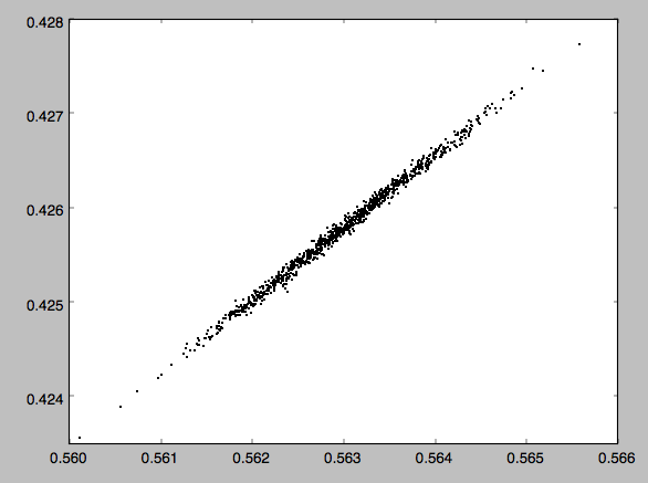
>>> sdf.plotCompareTrackAAModel()

which in this case gives

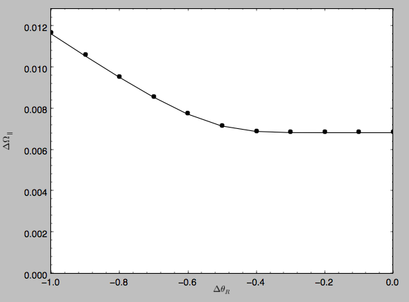
This displays the stream model’s track in frequency offset (y axis) versus angle offset (x axis) as the solid line; this is the track that the model should have if it is calculated correctly. The points are the frequency and angle offset calculated from the calculated track’s \((\mathbf{x},\mathbf{v})\). For a properly computed track these should line up, as they do in this figure. If they do not line up, increasing nTrackIterations is necessary.

We can calculate some simple properties of the stream, such as the ratio of the largest and second-to-largest eigenvalue of the Hessian \(\partial \mathbf{\Omega} / \partial \mathbf{J}\)

>>> sdf.freqEigvalRatio(isotropic=True)
# 34.450028399901434

or the model’s ratio of the largest and second-to-largest eigenvalue of the model frequency variance matrix

>>> sdf.freqEigvalRatio()
# 29.625538344985291

The fact that this ratio is so large means that an approximately one dimensional stream will form.

Similarly, we can calculate the angle between the frequency vector of the progenitor and of the model mean frequency vector

>>> sdf.misalignment()
# 0.0086441947505973005

which returns this angle in radians. We can also calculate the angle between the frequency vector of the progenitor and the principal eigenvector of \(\partial \mathbf{\Omega} / \partial \mathbf{J}\)

>>> sdf.misalignment(isotropic=True)
# 0.02238411611147997

(the reason these are obtained by specifying isotropic=True is that these would be the ratio of the eigenvalues or the angle if we assumed that the disrupted materials action distribution were isotropic).

Calculating the average stream location (track)

We can display the stream track in various coordinate systems as follows

>>> sdf.plotTrack(d1='r',d2='z',interp=True,color='k',spread=2,overplot=False,lw=2.,scaleToPhysical=True)

which gives

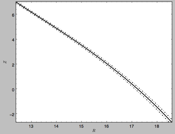
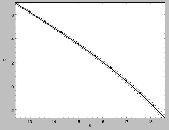
which shows the track in Galactocentric R and Z coordinates as well as an estimate of the spread around the track as the dash-dotted line. We can overplot the points along the track along which the \((\mathbf{x},\mathbf{v}) \rightarrow (\mathbf{\Omega},\boldsymbol{\theta})\) transformation and the track position is explicitly calculated, by turning off the interpolation

>>> sdf.plotTrack(d1='r',d2='z',interp=False,color='k',spread=0,overplot=True,ls='none',marker='o',scaleToPhysical=True)

which gives

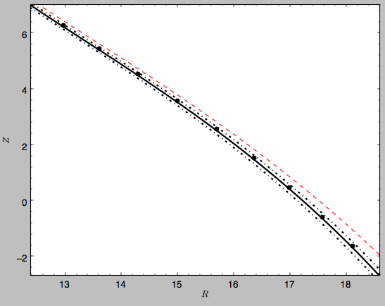
We can also overplot the orbit of the progenitor

>>> sdf.plotProgenitor(d1='r',d2='z',color='r',overplot=True,ls='--',scaleToPhysical=True)

to give

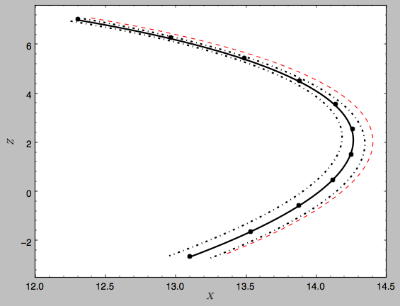
We can do the same in other coordinate systems, for example X and Z (as in Figure 1 of Bovy 2014)

>>> sdf.plotTrack(d1='x',d2='z',interp=True,color='k',spread=2,overplot=False,lw=2.,scaleToPhysical=True)
>>> sdf.plotTrack(d1='x',d2='z',interp=False,color='k',spread=0,overplot=True,ls='none',marker='o',scaleToPhysical=True)
>>> sdf.plotProgenitor(d1='x',d2='z',color='r',overplot=True,ls='--',scaleToPhysical=True)
>>> xlim(12.,14.5); ylim(-3.5,7.6)

which gives

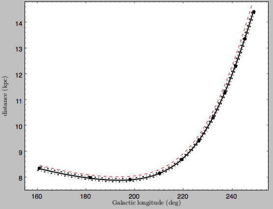
or we can calculate the track in observable coordinates, e.g.,

>>> sdf.plotTrack(d1='ll',d2='dist',interp=True,color='k',spread=2,overplot=False,lw=2.)
>>> sdf.plotTrack(d1='ll',d2='dist',interp=False,color='k',spread=0,overplot=True,ls='none',marker='o')
>>> sdf.plotProgenitor(d1='ll',d2='dist',color='r',overplot=True,ls='--')
>>> xlim(155.,255.); ylim(7.5,14.8)

which displays

Coordinate transformations to physical coordinates are done using parameters set when initializing the sdf instance. See the help for ?streamdf for a complete list of initialization parameters.

Mock stream data generation

We can also easily generate mock data from the stream model. This uses streamdf.sample. For example,

>>> RvR= sdf.sample(n=1000)

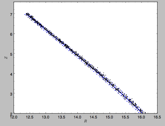
which returns the sampled points as a set \((R,v_R,v_T,Z,v_Z,\phi)\) in natural galpy coordinates. We can plot these and compare them to the track location

>>> sdf.plotTrack(d1='r',d2='z',interp=True,color='b',spread=2,overplot=False,lw=2.,scaleToPhysical=True)
>>> plot(RvR[0]*8.,RvR[3]*8.,'k.',ms=2.) #multiply by the physical distance scale
>>> xlim(12.,16.5); ylim(2.,7.6)

which gives

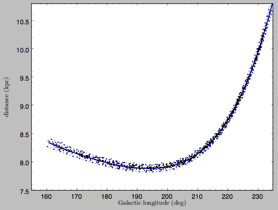
Similarly, we can generate mock data in observable coordinates

>>> lb= sdf.sample(n=1000,lb=True)

and plot it

>>> sdf.plotTrack(d1='ll',d2='dist',interp=True,color='b',spread=2,overplot=False,lw=2.)
>>> plot(lb[0],lb[2],'k.',ms=2.)
>>> xlim(155.,235.); ylim(7.5,10.8)

which displays

We can also just generate mock stream data in frequency-angle coordinates

>>> mockaA= sdf.sample(n=1000,returnaAdt=True)

which returns a tuple with three components: an array with shape [3,N] of frequency vectors \((\Omega_R,\Omega_\phi,\Omega_Z)\), an array with shape [3,N] of angle vectors \((\theta_R,\theta_\phi,\theta_Z)\) and \(t_s\), the stripping time. We can plot the vertical versus the radial frequency

>>> plot(mockaA[0][0],mockaA[0][2],'k.',ms=2.)

or we can plot the magnitude of the angle offset as a function of stripping time

>>> plot(mockaA[2],numpy.sqrt(numpy.sum((mockaA[1]-numpy.tile(sdf._progenitor_angle,(1000,1)).T)**2.,axis=0)),'k.',ms=2.)

Evaluating and marginalizing the full PDF

We can also evaluate the stream PDF, the probability of a \((\mathbf{x},\mathbf{v})\) phase-space position in the stream. We can evaluate the PDF, for example, at the location of the progenitor

>>> sdf(obs.R(),obs.vR(),obs.vT(),obs.z(),obs.vz(),obs.phi())
# array([-33.16985861])

which returns the natural log of the PDF. If we go slightly higher in Z and slightly smaller in R, the PDF becomes zero

>>> sdf(obs.R()-0.1,obs.vR(),obs.vT(),obs.z()+0.1,obs.vz(),obs.phi())
# array([-inf])

because this phase-space position cannot be reached by a leading stream star. We can also marginalize the PDF over unobserved directions. For example, similar to Figure 10 in Bovy (2014), we can evaluate the PDF \(p(X|Z)\) near a point on the track, say near Z =2 kpc (=0.25 in natural units. We first find the approximate Gaussian PDF near this point, calculated from the stream track and dispersion (see above)

>>> meanp, varp= sdf.gaussApprox([None,None,2./8.,None,None,None])

where the input is a array with entries [X,Y,Z,vX,vY,vZ] and we substitute None for directions that we want to establish the approximate PDF for. So the above expression returns an approximation to \(p(X,Y,v_X,v_Y,v_Z|Z)\). This approximation allows us to get a sense of where the PDF peaks and what its width is

>>> meanp[0]*8.
# 14.267559400127833
>>> numpy.sqrt(varp[0,0])*8.
# 0.04152968631186698

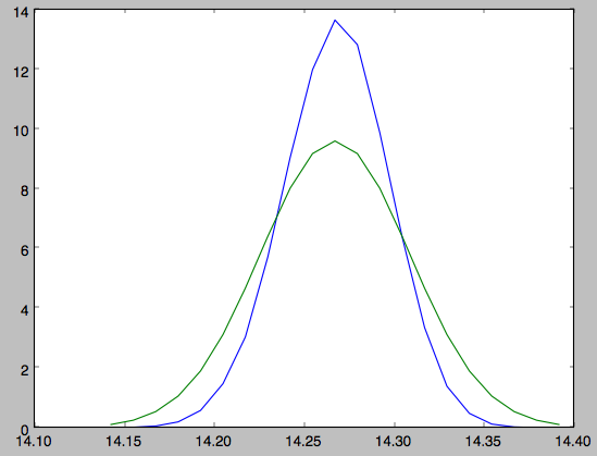
We can now evaluate the PDF \(p(X|Z)\) as a function of X near the peak

>>> xs= numpy.linspace(-3.*numpy.sqrt(varp[0,0]),3.*numpy.sqrt(varp[0,0]),21)+meanp[0]
>>> logps= numpy.array([sdf.callMarg([x,None,2./8.,None,None,None]) for x in xs])
>>> ps= numpy.exp(logps)

and we normalize the PDF

>>> ps/= numpy.sum(ps)*(xs[1]-xs[0])*8.

and plot it together with the Gaussian approximation

>>> plot(xs*8.,ps)
>>> plot(xs*8.,1./numpy.sqrt(2.*numpy.pi)/numpy.sqrt(varp[0,0])/8.*numpy.exp(-0.5*(xs-meanp[0])**2./varp[0,0]))

which gives

Sometimes it is hard to automatically determine the closest point on the calculated track if only one phase-space coordinate is given. For example, this happens when evaluating \(p(Z|X)\) for X > 13 kpc here, where there are two branches of the track in Z (see the figure of the track above). In that case, we can determine the closest track point on one of the branches by hand and then provide this closest point as the basis of PDF calculations. The following example shows how this is done for the upper Z branch at X = 13.5 kpc, which is near Z =5 kpc (Figure 10 in Bovy 2014).

>>> cindx= sdf.find_closest_trackpoint(13.5/8.,None,5.32/8.,None,None,None,xy=True)

gives the index of the closest point on the calculated track. This index can then be given as an argument for the PDF functions:

>>> meanp, varp= meanp, varp= sdf.gaussApprox([13.5/8.,None,None,None,None,None],cindx=cindx)

computes the approximate \(p(Y,Z,v_X,v_Y,v_Z|X)\) near the upper Z branch. In Z, this PDF has mean and dispersion

>>> meanp[1]*8.
# 5.4005530328542077
>>> numpy.sqrt(varp[1,1])*8.
# 0.05796023309510244

We can then evaluate \(p(Z|X)\) for the upper branch as

>>> zs= numpy.linspace(-3.*numpy.sqrt(varp[1,1]),3.*numpy.sqrt(varp[1,1]),21)+meanp[1]
>>> logps= numpy.array([sdf.callMarg([13.5/8.,None,z,None,None,None],cindx=cindx) for z in zs])
>>> ps= numpy.exp(logps)
>>> ps/= numpy.sum(ps)*(zs[1]-zs[0])*8.

and we can again plot this and the approximation

>>> plot(zs*8.,ps)
>>> plot(zs*8.,1./numpy.sqrt(2.*numpy.pi)/numpy.sqrt(varp[1,1])/8.*numpy.exp(-0.5*(zs-meanp[1])**2./varp[1,1]))

which gives

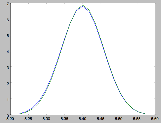
The approximate PDF in this case is very close to the correct PDF. When supplying the closest track point, care needs to be taken that this really is the closest track point. Otherwise the approximate PDF will not be quite correct.

Modeling gaps in streams using action-angle coordinates

galpy also contains tools to model the effect of impacts due to dark-matter subhalos on streams (see Sanders, Bovy, & Erkal 2015). This is implemented as a subclass streamgapdf of streamdf, because they share many of the same methods. Setting up a streamgapdf object requires the same arguments and keywords as setting up a streamdf instance (to specify the smooth underlying stream model and the Galactic potential) as well as parameters that specify the impact (impact parameter and velocity, location and time of closest approach, mass and structure of the subhalo, and helper keywords that specify how the impact should be calculated). An example used in the paper (but not that with the modifications in Sec. 6.1) is as follows. Imports:

>>> from galpy.df import streamdf, streamgapdf
>>> from galpy.orbit import Orbit
>>> from galpy.potential import LogarithmicHaloPotential
>>> from galpy.actionAngle import actionAngleIsochroneApprox
>>> from galpy.util import conversion

Parameters for the smooth stream and the potential:

>>> lp= LogarithmicHaloPotential(normalize=1.,q=0.9)
>>> aAI= actionAngleIsochroneApprox(pot=lp,b=0.8)
>>> prog_unp_peri= Orbit([2.6556151742081835,
                          0.2183747276300308,
                          0.67876510797240575,
                          -2.0143395648974671,
                          -0.3273737682604374,
                          0.24218273922966019])
>>> V0, R0= 220., 8.
>>> sigv= 0.365*(10./2.)**(1./3.) # km/s
>>> tdisrupt= 10.88/conversion.time_in_Gyr(V0,R0)

and the parameters of the impact

>>> GM= 10.**-2./conversion.mass_in_1010msol(V0,R0)
>>> rs= 0.625/R0
>>> impactb= 0.
>>> subhalovel= numpy.array([6.82200571,132.7700529,149.4174464])/V0
>>> timpact= 0.88/conversion.time_in_Gyr(V0,R0)
>>> impact_angle= -2.34

The setup is then

>>> sdf_sanders15= streamgapdf(sigv/V0,progenitor=prog_unp_peri,pot=lp,aA=aAI,
                               leading=False,nTrackChunks=26,
                               nTrackIterations=1,
                               sigMeanOffset=4.5,
                               tdisrupt=tdisrupt,
                               Vnorm=V0,Rnorm=R0,
                               impactb=impactb,
                               subhalovel=subhalovel,
                               timpact=timpact,
                               impact_angle=impact_angle,
                               GM=GM,rs=rs)

The streamgapdf implementation is currently not entirely complete (for example, one cannot yet evaluate the full phase-space PDF), but the model can be sampled as in the paper above. To compare the perturbed model to the unperturbed model, we also set up an unperturbed model of the same stream

>>> sdf_sanders15_unp= streamdf(sigv/V0,progenitor=prog_unp_peri,pot=lp,aA=aAI,
                               leading=False,nTrackChunks=26,
                               nTrackIterations=1,
                               sigMeanOffset=4.5,
                               tdisrupt=tdisrupt,
                               Vnorm=V0,Rnorm=R0)

We can then sample positions and velocities for the perturbed and unperturbed preduction for the same particle by using the same random seed:

>>> numpy.random.seed(1)
>>> xv_mock_per= sdf_sanders15.sample(n=100000,xy=True).T
>>> numpy.random.seed(1) # should give same points
>>> xv_mock_unp= sdf_sanders15_unp.sample(n=100000,xy=True).T

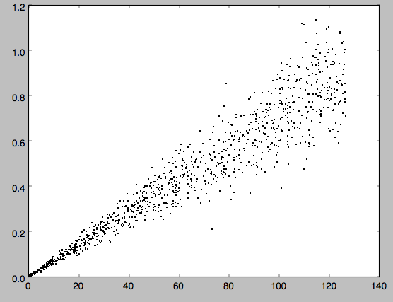
and we can plot the offset due to the perturbation, for example,

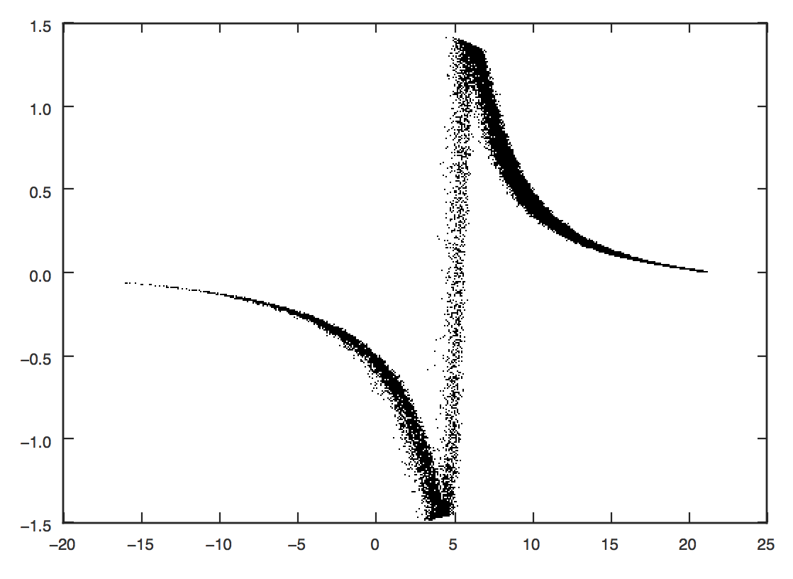
>>> plot(xv_mock_unp[:,0]*R0,(xv_mock_per[:,0]-xv_mock_unp[:,0])*R0,'k,')

for the difference in \(X\) as a function of unperturbed \(X\):

or

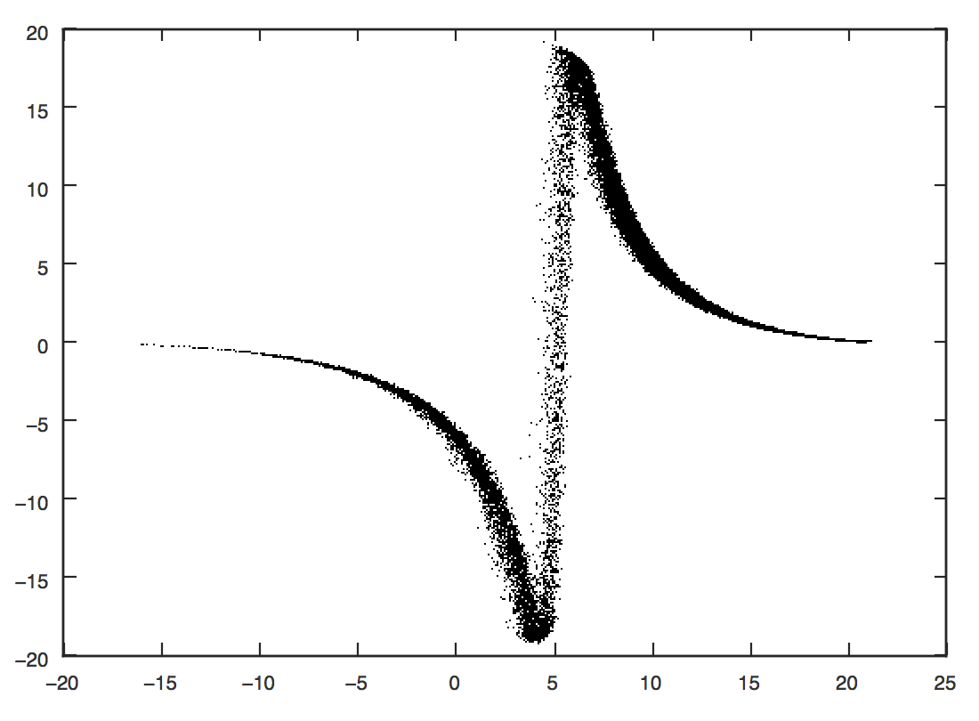
>>> plot(xv_mock_unp[:,0]*R0,(xv_mock_per[:,4]-xv_mock_unp[:,4])*V0,'k,')

for the difference in \(v_Y\) as a function of unperturbed \(X\):

Particle-spray modeling of streams with streamspraydf

galpy also contains an implementation of the particle-spray method for generating tidal streams, roughly following the parametrization of Fardal et al. (2015). Full details on the galpy implementation are given in Qian et al. (2022). Here, we give a simple example of the method.

Like in the streamdf example above, we use the same orbit, potential, and cluster mass as in Bovy (2014). We setup the orbit of the progenitor and the gravitational potential (modeled as a simple LogarithmicHaloPotential):

>>> from galpy.potential import LogarithmicHaloPotential
>>> from galpy.orbit import Orbit
>>> o= Orbit([1.56148083,0.35081535,-1.15481504,0.88719443,-0.47713334,0.12019596])
>>> lp= LogarithmicHaloPotential(normalize=1.,q=0.9)

Then, we setup streamspraydf models for the leading and trailing arm of the stream:

>>> from astropy import units
>>> from galpy.df import streamspraydf
>>> spdf= streamspraydf(2*10.**4.*units.Msun,progenitor=o,pot=lp,tdisrupt=4.5*units.Gyr)
>>> spdft= streamspraydf(2*10.**4.*units.Msun,progenitor=o,pot=lp,leading=False,tdisrupt=4.5*units.Gyr)

To sample a set of 300 stars in both arms, we do

>>> orbs,dt= spdf.sample(n=300,returndt=True,integrate=True)
>>> orbts,dt= spdft.sample(n=300,returndt=True,integrate=True)

which returns a galpy.orbit.Orbit instance with all 300 stars. We can plot these in \(Z\) versus \(X\) and compare to Fig. 1 in Bovy (2014). First, we also integrate the orbit of the progenitor forward and backward in time for a brief period to show its location in the area of the stream:

>>> ts= numpy.linspace(0.,3.,301)
>>> o.integrate(ts,lp)
>>> of= o()
>>> of.integrate(-ts,lp)

Then we plot

>>> o.plot(d1='x',d2='z',color='k',xrange=[0.,2.],yrange=[-0.1,1.45])
>>> of.plot(d1='x',d2='z',overplot=True,color='k')
>>> plot(orbs.x(),orbs.z(),'r.')
>>> plot(orbts.x(),orbts.z(),'b.')

which gives

We can also compare to the track for this stream as predicted by streamdf. For this, we first setup a similar streamdf model (they are not exactly the same, as streamdf uses a velocity dispersion to set the progenitor’s mass, while streamspraydf uses the mass directly); see the streamdf documentation for a full explanation of this code:

>>> from galpy.actionAngle import actionAngleIsochroneApprox
>>> from galpy.df import streamdf
>>> aAIA= actionAngleIsochroneApprox(b=0.8,pot=lp)
>>> sigv= 0.365 #km/s
>>> sdf= streamdf(sigv/220.,progenitor=o(),pot=lp,aA=aAIA,leading=True,
                  nTrackChunks=11,tdisrupt=4.5*units.Gyr)
>>> sdft= streamdf(sigv/220.,progenitor=o(),pot=lp,aA=aAIA,leading=False,
                   nTrackChunks=11,tdisrupt=4.5*units.Gyr)

Then, we can overplot the track predicted by streamdf:

>>> o.plot(d1='x',d2='z',color='k',xrange=[0.,2.],yrange=[-0.1,1.45])
>>> of.plot(d1='x',d2='z',overplot=True,color='k')
>>> plot(orbs.x(),orbs.z(),'r.',alpha=0.1)
>>> plot(orbts.x(),orbts.z(),'b.',alpha=0.1)
>>> sdf.plotTrack(d1='x',d2='z',interp=True,color='r',overplot=True,lw=1.)
>>> sdft.plotTrack(d1='x',d2='z',interp=True,color='b',overplot=True,lw=1.)

This gives then

We see that the track from streamdf agrees very well with the location of the points sampled from streamspraydf.

The streamspraydf sample function can also return the points at the time of stripping, that is, not integrated to the present time (when using integrate=False); this can be useful for visualizing where stars get stripped from the progenitor. When initializing streamspraydf, you can also specify a different potential for computing the tidal radius and velocity distribution of the tidal debris, which can be useful when the overall potential contains pieces that are irrelevant for computing the tidal radius and that don’t allow the tidal radius to be computed (using the rtpot= option). If you want to generate a stream around a moving object, for example, a stream created within a satellite galaxy of the Milky Way, you can specify an orbit for the center of the satellite (center=) and the stream will be generated around this center rather than around the center of the total potential (this was used in Qian et al. 2022); the center orbit is integrated in centerpot, which can also differ from the potential that stream stars are integrated in (e.g., the stream stars may feel the potential from the satellite itself and/or the satellite could be experiencing dynamical friction which the stream stars do not feel).