Three-dimensional disk distribution functions

galpy contains a fully three-dimensional disk distribution: galpy.df.quasiisothermaldf, which is an approximately isothermal distribution function expressed in terms of action–angle variables (see 2010MNRAS.401.2318B and 2011MNRAS.413.1889B). Recent research shows that this distribution function provides a good model for the DF of mono-abundance sub-populations (MAPs) of the Milky Way disk (see 2013MNRAS.434..652T and 2013ApJ…779..115B). This distribution function family requires action-angle coordinates to evaluate the DF, so galpy.df.quasiisothermaldf makes heavy use of the routines in galpy.actionAngle (in particular those in galpy.actionAngleAdiabatic and galpy.actionAngle.actionAngleStaeckel).

Setting up the DF and basic properties

The quasi-isothermal DF is defined by a gravitational potential and a set of parameters describing the radial surface-density profile and the radial and vertical velocity dispersion as a function of radius. In addition, we have to provide an instance of a galpy.actionAngle class to calculate the actions for a given position and velocity. For example, for a galpy.potential.MWPotential2014 potential using the adiabatic approximation for the actions, we import and define the following

>>> from galpy.potential import MWPotential2014
>>> from galpy.actionAngle import actionAngleAdiabatic
>>> from galpy.df import quasiisothermaldf
>>> aA= actionAngleAdiabatic(pot=MWPotential2014,c=True)

and then setup the quasiisothermaldf instance

>>> qdf= quasiisothermaldf(1./3.,0.2,0.1,1.,1.,pot=MWPotential2014,aA=aA,cutcounter=True)

which sets up a DF instance with a radial scale length of \(R_0/3\), a local radial and vertical velocity dispersion of \(0.2\,V_c(R_0)\) and \(0.1\,V_c(R_0)\), respectively, and a radial scale lengths of the velocity dispersions of \(R_0\). cutcounter=True specifies that counter-rotating stars are explicitly excluded (normally these are just exponentially suppressed). As for the two-dimensional disk DFs, these parameters are merely input (or target) parameters; the true density and velocity dispersion profiles calculated by evaluating the relevant moments of the DF (see below) are not exactly exponential and have scale lengths and local normalizations that deviate slightly from these input parameters. We can estimate the DF’s actual radial scale length near \(R_0\) as

>>> qdf.estimate_hr(1.)
# 0.32908034635647182

which is quite close to the input value of 1/3. Similarly, we can estimate the scale lengths of the dispersions

>>> qdf.estimate_hsr(1.)
# 1.1913935820372923
>>> qdf.estimate_hsz(1.)
# 1.0506918075359255

The vertical profile is fully specified by the velocity dispersions and radial density / dispersion profiles under the assumption of dynamical equilibrium. We can estimate the scale height of this DF at a given radius and height as follows

>>> qdf.estimate_hz(1.,0.125)
# 0.021389597757156088

Near the mid-plane this vertical scale height becomes very large because the vertical profile flattens, e.g.,

>>> qdf.estimate_hz(1.,0.125/100.)
# 1.006386030587223

or even

>>> qdf.estimate_hz(1.,0.)
# 221852.19839263527

which is basically infinity.

Evaluating moments

We can evaluate various moments of the DF giving the density, mean velocities, and velocity dispersions. For example, the mean radial velocity is again everywhere zero because the potential and the DF are axisymmetric

>>> qdf.meanvR(1.,0.)
# 0.0

Likewise, the mean vertical velocity is everywhere zero

>>> qdf.meanvz(1.,0.)
# 0.0

The mean rotational velocity has a more interesting dependence on position. Near the plane, this is the same as that calculated for a similar two-dimensional disk DF (see Evaluating moments of the DF)

>>> qdf.meanvT(1.,0.)
# 0.91988346380781227

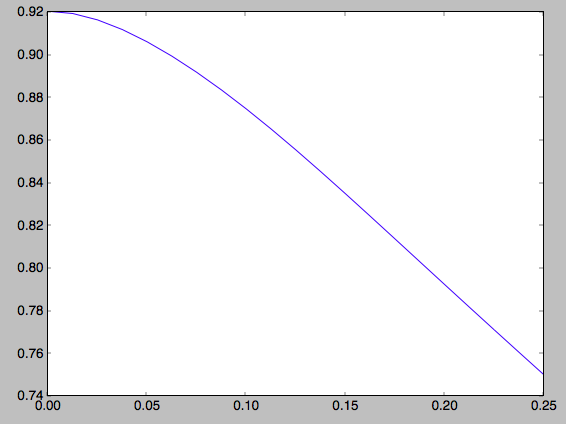
However, this value decreases as one moves further from the plane. The quasiisothermaldf allows us to calculate the average rotational velocity as a function of height above the plane. For example,

>>> zs= numpy.linspace(0.,0.25,21)
>>> mvts= numpy.array([qdf.meanvT(1.,z) for z in zs])

which gives

>>> plot(zs,mvts)

We can also calculate the second moments of the DF. We can check whether the radial and velocity dispersions at \(R_0\) are close to their input values

>>> numpy.sqrt(qdf.sigmaR2(1.,0.))
# 0.20807112565801389
>>> numpy.sqrt(qdf.sigmaz2(1.,0.))
# 0.090453510526130904

and they are pretty close. We can also calculate the mixed R and z moment, for example,

>>> qdf.sigmaRz(1.,0.125)
# 0.0

or expressed as an angle (the tilt of the velocity ellipsoid)

>>> qdf.tilt(1.,0.125)
# 0.0

This tilt is zero because we are using the adiabatic approximation. As this approximation assumes that the motions in the plane are decoupled from the vertical motions of stars, the mixed moment is zero. However, this approximation is invalid for stars that go far above the plane. By using the Staeckel approximation to calculate the actions, we can model this coupling better. Setting up a quasiisothermaldf instance with the Staeckel approximation

>>> from galpy.actionAngle import actionAngleStaeckel
>>> aAS= actionAngleStaeckel(pot=MWPotential2014,delta=0.45,c=True)
>>> qdfS= quasiisothermaldf(1./3.,0.2,0.1,1.,1.,pot=MWPotential2014,aA=aAS,cutcounter=True)

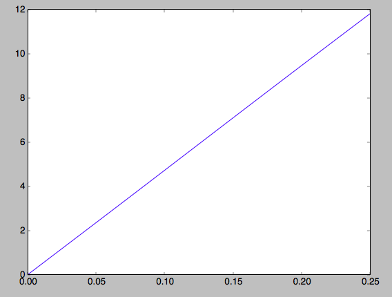
we can similarly calculate the tilt

>>> qdfS.tilt(1.,0.125)
# 0.10314272868452541

or about 5 degrees (the returned value has units of rad). As a function of height, we find

>>> tilts= numpy.array([qdfS.tilt(1.,z) for z in zs])
>>> plot(zs,tilts*180./numpy.pi)

which gives

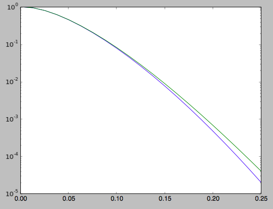
We can also calculate the density and surface density (the zero-th velocity moments). For example, the vertical density

>>> densz= numpy.array([qdf.density(1.,z) for z in zs])

and

>>> denszS= numpy.array([qdfS.density(1.,z) for z in zs])

We can compare the vertical profiles calculated using the adiabatic and Staeckel action-angle approximations

>>> semilogy(zs,densz/densz[0])
>>> semilogy(zs,denszS/denszS[0])

which gives

Similarly, we can calculate the radial profile of the surface density

>>> rs= numpy.linspace(0.5,1.5,21)
>>> surfr= numpy.array([qdf.surfacemass_z(r) for r in rs])
>>> surfrS= numpy.array([qdfS.surfacemass_z(r) for r in rs])

and compare them with each other and an exponential with scale length 1/3

>>> semilogy(rs,surfr/surfr[10])
>>> semilogy(rs,surfrS/surfrS[10])
>>> semilogy(rs,numpy.exp(-(rs-1.)/(1./3.)))

which gives

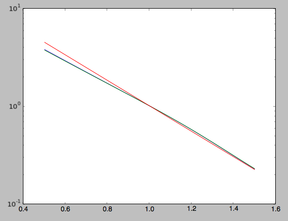
The two radial profiles are almost indistinguishable and are very close, if somewhat shallower, than the pure exponential profile.

General velocity moments, including all higher order moments, are implemented in quasiisothermaldf.vmomentdensity.

Evaluating and sampling the full probability distribution function

We can evaluate the distribution itself by calling the object, e.g.,

>>> qdf(1.,0.1,1.1,0.1,0.) #input: R,vR,vT,z,vz
# array([ 16.86790643])

or as a function of rotational velocity, for example in the mid-plane

>>> vts= numpy.linspace(0.,1.5,101)
>>> pvt= numpy.array([qdfS(1.,0.,vt,0.,0.) for vt in vts])
>>> plot(vts,pvt/numpy.sum(pvt)/(vts[1]-vts[0]))

which gives

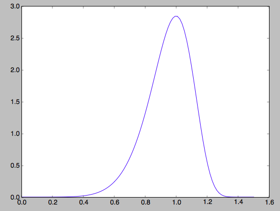
This is, however, not the true distribution of rotational velocities at R =0 and z =0, because it is conditioned on zero radial and vertical velocities. We can calculate the distribution of rotational velocities marginalized over the radial and vertical velocities as

>>> qdfS.pvT(1.,1.,0.) #input vT,R,z
# 58.708924787596544

or as a function of rotational velocity

>>> pvt= numpy.array([qdfS.pvT(vt,1.,0.) for vt in vts])

overplotting this over the previous distribution gives

>>> plot(vts,pvt/numpy.sum(pvt)/(vts[1]-vts[0]))

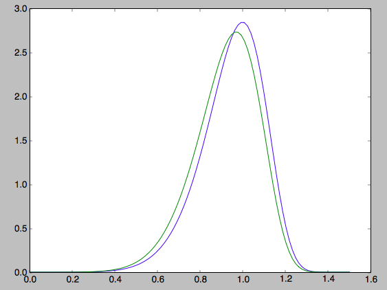
which is slightly different from the conditioned distribution. Similarly, we can calculate marginalized velocity probabilities pvR, pvz, pvRvT, pvRvz, and pvTvz. These are all multiplied with the density, such that marginalizing these over the remaining velocity component results in the density.

We can sample velocities at a given location using quasiisothermaldf.sampleV (there is currently no support for sampling locations from the density profile, although that is rather trivial):

>>> vs= qdfS.sampleV(1.,0.,n=10000)
>>> hist(vs[:,1],density=True,histtype='step',bins=101,range=[0.,1.5])

gives

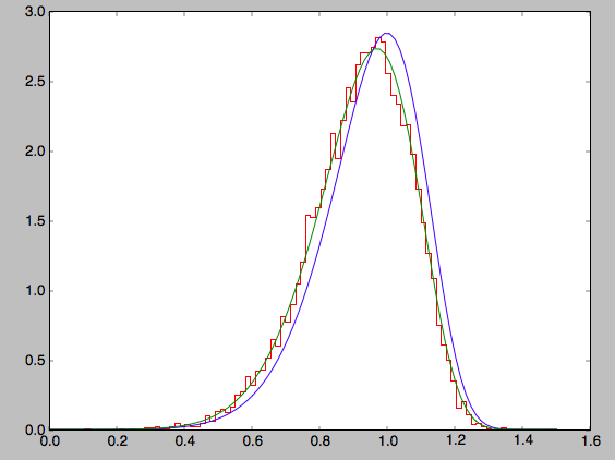
which shows very good agreement with the green (marginalized over vR and vz) curve (as it should).