Potentials in galpy
galpy contains a large variety of potentials in galpy.potential
that can be used for orbit integration, the calculation of
action-angle coordinates, as part of steady-state distribution
functions, and to study the properties of gravitational
potentials. This section introduces some of these features.
Potentials and forces
Various 3D and 2D potentials are contained in galpy, list in the API page. Another way to list the latest overview of potentials included with galpy is to run
>>> import galpy.potential
>>> print([p for p in dir(galpy.potential) if 'Potential' in p])
# ['CosmphiDiskPotential',
#  'DehnenBarPotential',
#  'DoubleExponentialDiskPotential',
#  'EllipticalDiskPotential',
#  'FlattenedPowerPotential',
#  'HernquistPotential',
# ....]
(list cut here for brevity). Section Rotation curves explains how to initialize potentials and how to display the rotation curve of single Potential instances or of combinations of such instances. Similarly, we can evaluate a Potential instance
>>> from galpy.potential import MiyamotoNagaiPotential
>>> mp= MiyamotoNagaiPotential(a=0.5,b=0.0375,normalize=1.)
>>> mp(1.,0.)
# -1.2889062500000001
Most member functions of Potential instances have corresponding
functions in the galpy.potential module that allow them to be
evaluated for lists of multiple Potential instances (and in versions
>=1.4 even for nested lists of Potential
instances). galpy.potential.MWPotential2014 is such a list of
three Potential instances
>>> from galpy.potential import MWPotential2014
>>> print(MWPotential2014)
# [<galpy.potential.PowerSphericalPotentialwCutoff.PowerSphericalPotentialwCutoff instance at 0x1089b23b0>, <galpy.potential.MiyamotoNagaiPotential.MiyamotoNagaiPotential instance at 0x1089b2320>, <galpy.potential.TwoPowerSphericalPotential.NFWPotential instance at 0x1089b2248>]
and we can evaluate the potential by using the evaluatePotentials
function
>>> from galpy.potential import evaluatePotentials
>>> evaluatePotentials(MWPotential2014,1.,0.)
# -1.3733506513947895
Tip
Lists of Potential instances can be nested, allowing you to easily add components to existing gravitational-potential models. For example, to add a DehnenBarPotential to MWPotential2014, you can do: pot= [MWPotential2014,DehnenBarPotential()] and then use this pot everywhere where you can use a list of Potential instances. You can also add potential simply as pot= MWPotential2014+DehnenBarPotential().
Warning
galpy potentials do not necessarily approach zero at infinity. To compute, for example, the escape velocity or whether or not an orbit is unbound, you need to take into account the value of the potential at infinity. E.g., \(v_{\mathrm{esc}}(r) = \sqrt{2[\Phi(\infty)-\Phi(r)]}\). If you want to create a potential that does go to zero at infinity, you can add a NullPotential with value equal to minus the original potential evaluated at infinity.
Tip
As discussed in the section on physical units, potentials can be initialized and evaluated with arguments specified as a astropy Quantity with units. Use the configuration parameter apy-units = True to get output values as a Quantity. See also the subsection on Initializing potentials with parameters with units below.
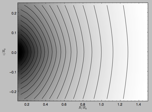
We can plot the potential of axisymmetric potentials (or of
non-axisymmetric potentials at phi=0) using the plot member
function
>>> mp.plot()
which produces the following plot
Similarly, we can plot combinations of Potentials using
plotPotentials, e.g.,
>>> from galpy.potential import plotPotentials
>>> plotPotentials(MWPotential2014,rmin=0.01)
These functions have arguments that can provide custom R and z
ranges for the plot, the number of grid points, the number of
contours, and many other parameters determining the appearance of
these figures.
galpy also allows the forces corresponding to a gravitational potential to be calculated. Again for the Miyamoto-Nagai Potential instance from above
>>> mp.Rforce(1.,0.)
# -1.0
This value of -1.0 is due to the normalization of the potential such that the circular velocity is 1. at R=1. Similarly, the vertical force is zero in the mid-plane
>>> mp.zforce(1.,0.)
# -0.0
but not further from the mid-plane
>>> mp.zforce(1.,0.125)
# -0.53488743705310848
As explained in Units in galpy, these forces are in
standard galpy units, and we can convert them to physical units using
methods in the galpy.util.conversion module. For example,
assuming a physical circular velocity of 220 km/s at R=8 kpc
>>> from galpy.util import conversion
>>> mp.zforce(1.,0.125)*conversion.force_in_kmsMyr(220.,8.)
# -3.3095671288657584 #km/s/Myr
>>> mp.zforce(1.,0.125)*conversion.force_in_2piGmsolpc2(220.,8.)
# -119.72021771473301 #2 \pi G Msol / pc^2
Again, there are functions in galpy.potential that allow for the
evaluation of the forces for lists of Potential instances, such that
>>> from galpy.potential import evaluateRforces
>>> evaluateRforces(MWPotential2014,1.,0.)
# -1.0
>>> from galpy.potential import evaluatezforces
>>> evaluatezforces(MWPotential2014,1.,0.125)*conversion.force_in_2piGmsolpc2(220.,8.)
>>> -69.680720137571114 #2 \pi G Msol / pc^2
We can evaluate the flattening of the potential as \(\sqrt{|z\,F_R/R\,F_Z|}\) for a Potential instance as well as for a list of such instances
>>> mp.flattening(1.,0.125)
# 0.4549542914935209
>>> from galpy.potential import flattening
>>> flattening(MWPotential2014,1.,0.125)
# 0.61231675305658628
Warning
While we call them ‘forces’ in galpy, the forces are really gravitational fields (forces per unit mass) or accelerations (through Newton’s second law).
Densities
galpy can also calculate the densities corresponding to gravitational potentials. For many potentials, the densities are explicitly implemented, but if they are not, the density is calculated using the Poisson equation (second derivatives of the potential have to be implemented for this). For example, for the Miyamoto-Nagai potential, the density is explicitly implemented
>>> mp.dens(1.,0.)
# 1.1145444383277576
and we can also calculate this using the Poisson equation
>>> mp.dens(1.,0.,forcepoisson=True)
# 1.1145444383277574
which are the same to machine precision
>>> mp.dens(1.,0.,forcepoisson=True)-mp.dens(1.,0.)
# -2.2204460492503131e-16
Similarly, all of the potentials in galpy.potential.MWPotential2014
have explicitly-implemented densities, so we can do
>>> from galpy.potential import evaluateDensities
>>> evaluateDensities(MWPotential2014,1.,0.)
# 0.57508603122264867
In physical coordinates, this becomes
>>> evaluateDensities(MWPotential2014,1.,0.)*conversion.dens_in_msolpc3(220.,8.)
# 0.1010945632524705 #Msol / pc^3
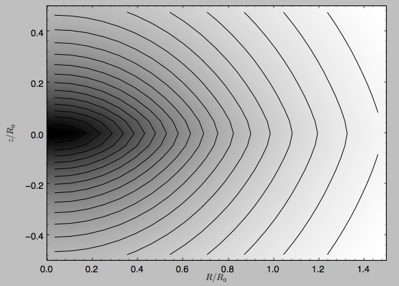
We can also plot densities
>>> from galpy.potential import plotDensities
>>> plotDensities(MWPotential2014,rmin=0.1,zmax=0.25,zmin=-0.25,nrs=101,nzs=101)
which gives
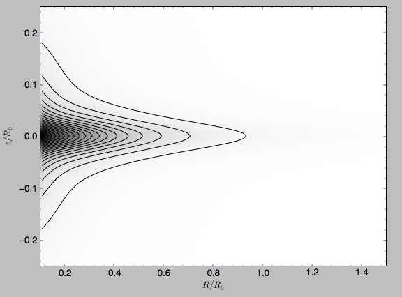
Another example of this is for an exponential disk potential
>>> from galpy.potential import DoubleExponentialDiskPotential
>>> dp= DoubleExponentialDiskPotential(hr=1./4.,hz=1./20.,normalize=1.)
The density computed using the Poisson equation now requires multiple numerical integrations, so the agreement between the analytical density and that computed using the Poisson equation is slightly less good, but still better than a percent
>>> (dp.dens(1.,0.,forcepoisson=True)-dp.dens(1.,0.))/dp.dens(1.,0.)
# 0.0032522956769123019
The density is
>>> dp.plotDensity(rmin=0.1,zmax=0.25,zmin=-0.25,nrs=101,nzs=101)
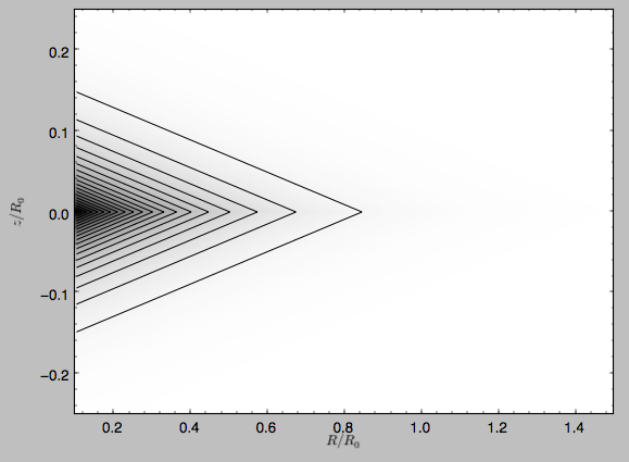
and the potential is
>>> dp.plot(rmin=0.1,zmin=-0.25,zmax=0.25)
Clearly, the potential is much less flattened than the density.
Modifying potential instances using wrappers
Potentials implemented in galpy can be modified using different kinds
of wrappers. These wrappers modify potentials to, for example, change
their amplitude as a function of time (e.g., to grow or decay the bar
contribution to a potential) or to make a potential rotate. Specific
kinds of wrappers are listed on the Potential wrapper API page. These wrappers can be applied to instances of any
potential implemented in galpy (including other wrappers). An example
is to grow a bar using the polynomial smoothing of Dehnen (2000). We first setup
an instance of a DehnenBarPotential that is essentially fully
grown already
>>> from galpy.potential import DehnenBarPotential
>>> dpn= DehnenBarPotential(tform=-100.,tsteady=0.) # DehnenBarPotential has a custom implementation of growth that we ignore by setting tform to -100
and then wrap it
>>> from galpy.potential import DehnenSmoothWrapperPotential
>>> dswp= DehnenSmoothWrapperPotential(pot=dpn,tform=-4.*2.*numpy.pi/dpn.OmegaP(),tsteady=2.*2.*numpy.pi/dpn.OmegaP())
This grows the DehnenBarPotential starting at 4 bar periods before
t=0 over a period of 2 bar periods. DehnenBarPotential has an
older, custom implementation of the same smoothing and the
(tform,tsteady) pair used here corresponds to the default setting
for DehnenBarPotential. Thus we can compare the two
>>> dp= DehnenBarPotential()
>>> print(dp(0.9,0.3,phi=3.,t=-2.)-dswp(0.9,0.3,phi=3.,t=-2.))
# 0.0
>>> print(dp.Rforce(0.9,0.3,phi=3.,t=-2.)-dswp.Rforce(0.9,0.3,phi=3.,t=-2.))
# 0.0
Other wrappers to modify the amplitude of a potential include
GaussianAmplitudeWrapperPotential, for modulating the amplitude using
a Gaussian, and the fully general TimeDependentAmplitudeWrapperPotential,
which can modulate the amplitude of any potential with an arbitrary function
of time.
Tip
To simply adjust the amplitude of a Potential instance, you can multiply the instance with a number or divide it by a number. For example, pot= 2.*LogarithmicHaloPotential(amp=1.) is equivalent to pot= LogarithmicHaloPotential(amp=2.). This is useful if you want to, for instance, quickly adjust the mass of a potential.
The wrapper SolidBodyRotationWrapperPotential allows one to make any potential rotate around the z axis. This can be used, for example, to make general bar-shaped potentials, which one could construct from a basis-function expansion with SCFPotential, rotate without having to implement the rotation directly. As an example consider this SoftenedNeedleBarPotential (which has a potential-specific implementation of rotation)
>>> sp= SoftenedNeedleBarPotential(normalize=1.,omegab=1.8,pa=0.)
The same potential can be obtained from a non-rotating SoftenedNeedleBarPotential run through the SolidBodyRotationWrapperPotential to add rotation
>>> sp_still= SoftenedNeedleBarPotential(omegab=0.,pa=0.,normalize=1.)
>>> swp= SolidBodyRotationWrapperPotential(pot=sp_still,omega=1.8,pa=0.)
Compare for example
>>> print(sp(0.8,0.2,phi=0.2,t=3.)-swp(0.8,0.2,phi=0.2,t=3.))
# 0.0
>>> print(sp.Rforce(0.8,0.2,phi=0.2,t=3.)-swp.Rforce(0.8,0.2,phi=0.2,t=3.))
# 8.881784197e-16
RotateAndTiltWrapperPotential is a wrapper that allows you to rotate,
tilt, or offset a potential. This can be useful if you are trying to
see a potential they way an external galaxy is tilted, or, in combination
with SolidBodyRotationWrapperPotential, to make a potential rotate around
an arbitrary axis (you can tilt, solid-body rotate, and tilt back to do this).
Wrapper potentials can be used anywhere in galpy where general
potentials can be used. They can be part of lists of Potential
instances. Wrappers can be wrapped again. They can also be used in C for
orbit integration provided that both the wrapper and the potentials that
it wraps are implemented in C. For example, a static LogarithmicHaloPotential
with a bar potential grown as above would be
>>> from galpy.potential import LogarithmicHaloPotential, evaluateRforces
>>> lp= LogarithmicHaloPotential(normalize=1.)
>>> pot= lp+dswp
>>> print(evaluateRforces(pot,0.9,0.3,phi=3.,t=-2.))
# -1.00965326579
Warning
When wrapping a potential that has physical outputs turned on, the wrapper object inherits the units of the wrapped potential and automatically turns them on, even when you do not explictly set ro= and vo=.
Close-to-circular orbits and orbital frequencies
We can also compute the properties of close-to-circular orbits. First of all, we can calculate the circular velocity and its derivative
>>> mp.vcirc(1.)
# 1.0
>>> mp.dvcircdR(1.)
# -0.163777427566978
or, for lists of Potential instances
>>> from galpy.potential import vcirc
>>> vcirc(MWPotential2014,1.)
# 1.0
>>> from galpy.potential import dvcircdR
>>> dvcircdR(MWPotential2014,1.)
# -0.10091361254334696
We can also calculate the various frequencies for close-to-circular orbits. For example, the rotational frequency
>>> mp.omegac(0.8)
# 1.2784598203204887
>>> from galpy.potential import omegac
>>> omegac(MWPotential2014,0.8)
# 1.2733514576122869
and the epicycle frequency
>>> mp.epifreq(0.8)
# 1.7774973530267848
>>> from galpy.potential import epifreq
>>> epifreq(MWPotential2014,0.8)
# 1.7452189766287691
as well as the vertical frequency
>>> mp.verticalfreq(1.0)
# 3.7859388972001828
>>> from galpy.potential import verticalfreq
>>> verticalfreq(MWPotential2014,1.)
# 2.7255405754769875
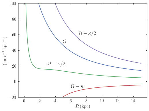
We can also for example easily make the diagram of \(\Omega-n
\kappa /m\) that is important for understanding kinematic spiral
density waves. For example, for MWPotential2014
>>> from galpy.potential import MWPotential2014, omegac, epifreq
>>> def OmegaMinusKappa(pot,Rs,n,m,ro=8.,vo=220.):
        # ro,vo for physical units, Rs in units of ro
        return omegac(pot,Rs/ro,ro=ro,vo=vo)-n/m*epifreq(pot,Rs/ro,ro=ro,vo=vo)
>>> Rs= numpy.linspace(0.,16.,101) # kpc
>>> plot(Rs,OmegaMinusKappa(MWPotential2014,Rs,0,1))
>>> plot(Rs,OmegaMinusKappa(MWPotential2014,Rs,1,2))
>>> plot(Rs,OmegaMinusKappa(MWPotential2014,Rs,1,1))
>>> plot(Rs,OmegaMinusKappa(MWPotential2014,Rs,1,-2))
>>> ylim(-20.,100.)
>>> xlabel(r'$R\,(\mathrm{kpc})$')
>>> ylabel(r'$(\mathrm{km\,s}^{-1}\,\mathrm{kpc}^{-1})$')
>>> text(3.,21.,r'$\Omega-\kappa/2$',size=18.)
>>> text(5.,50.,r'$\Omega$',size=18.)
>>> text(7.,60.,r'$\Omega+\kappa/2$',size=18.)
>>> text(6.,-7.,r'$\Omega-\kappa$',size=18.)
which gives
For close-to-circular orbits, we can also compute the radii of the Lindblad resonances. For example, for a frequency similar to that of the Milky Way’s bar
>>> mp.lindbladR(5./3.,m='corotation') #args are pattern speed and m of pattern
# 0.6027911166042229 #~ 5kpc
>>> print(mp.lindbladR(5./3.,m=2))
# None
>>> mp.lindbladR(5./3.,m=-2)
# 0.9906190683480501
The None here means that there is no inner Lindblad resonance, the
m=-2 resonance is in the Solar neighborhood (see the section on
the Hercules stream in this documentation).
Using interpolations of potentials
galpy contains various ways to set up interpolated versions of
potentials that can be used to generate interpolations of potentials
that can be used in their stead to speed up calculations when the
calculation of the original potential is computationally expensive
(for example, for the DoubleExponentialDiskPotential).
To interpolated spherical potentials, use the
interpSphericalPotential class, described in detail here. To set up an instance, simply provide a function that
gives the radial force as a function of (spherical) radius and a grid
to interpolate it over (to set up a potential for a given enclosed
mass, give the enclosed mass divided by radius
squared). Alternatively, provide a spherical galpy potential
instance or a list of such instances to build an interpolated version
of them.
To interpolate axisymmetric potentials, use the interpRZPotential
class. Full details on how to set this up are given here.
Interpolated potentials can be used anywhere that general
three-dimensional galpy potentials can be used. Some care must be
taken with outside-the-interpolation-grid evaluations for functions
that use C to speed up computations.
Initializing potentials with parameters with units
As already discussed in the section on physical units, potentials in galpy can be specified with parameters
with units since v1.2. For most inputs to the initialization it is
straightforward to know what type of units the input Quantity needs to
have. For example, the scale length parameter a= of a
Miyamoto-Nagai disk needs to have units of distance.
The amplitude of a potential is specified through the amp=
initialization parameter. The units of this parameter vary from
potential to potential. For example, for a logarithmic potential the
units are velocity squared, while for a Miyamoto-Nagai potential they
are units of mass. Check the documentation of each potential on the
API page for the units of the amp=
parameter of the potential that you are trying to initialize and
please report an Issue if
you find any problems with this.
UPDATED IN v1.8 General density/potential pairs with basis-function expansions
galpy allows for the potential and forces of general,
time-independent density functions to be computed by expanding the
potential and density in terms of basis functions. This is supported
for ellipsoidal-ish as well as for disk-y density distributions, in
both cases using the basis-function expansion of the
self-consistent-field (SCF) method of Hernquist & Ostriker (1992). On its own,
the SCF technique works well for ellipsoidal-ish density
distributions, but using a trick due to Kuijken & Dubinski (1995) it can also be
made to work well for disky potentials. We first describe the basic
SCF implementation and then discuss how to use it for disky
potentials.
The basis-function approach in the SCF method is implemented in the
SCFPotential class, which is also implemented
in C for fast orbit integration. The easiest way to initialize an
SCFPotential using a target density profile is using the
SCFPotential.from_density method. As an example, we consider a
prolate NFW potential
>>> from galpy.potential import TriaxialNFWPotential
>>> np= TriaxialNFWPotential(normalize=1.,c=1.4,a=1.)
To create an SCFPotential version of this, we need to chose a value of
a scale parameter a that is used in the definition of the basis functions
(this often needs to be tweaked to create the best-possible match with as
few basis functions as possible). Once we choose a value for a, we can
initialize the SCFPotential as follows
>>> a_SCF= 50. # much larger a than true scale radius works well for NFW
>>> from galpy.potential import SCFPotential
>>> sp= SCFPotential.from_density(np.dens,80,L=40,a=a_SCF,symmetry='axisymmetry')
Here symmetry='axisymmetry' indicates that we are assuming axisymmetry in the
basis-function expansion; other valid values are symmetry='spherical' when
assuming spherical symmetry or symmetry=None for the general, non-axisymmetric
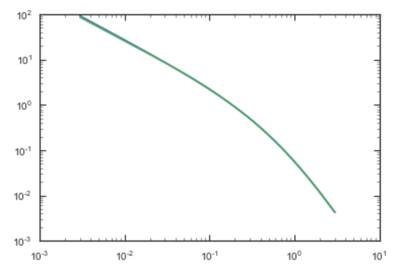
computation. If we compare the densities along the R=Z line as
>>> xs= numpy.linspace(0.,3.,1001)
>>> loglog(xs,[np.dens(x,x) for x in xs])
>>> loglog(xs,sp.dens(xs,xs))
we get
If we then integrate an orbit, we also get good agreement
>>> from galpy.orbit import Orbit
>>> o= Orbit([1.,0.1,1.1,0.1,0.3,0.])
>>> ts= numpy.linspace(0.,100.,10001)
>>> o.integrate(ts,np)
>>> o.plot()
>>> o.integrate(ts,sp)
>>> o.plot(overplot=True)
which gives
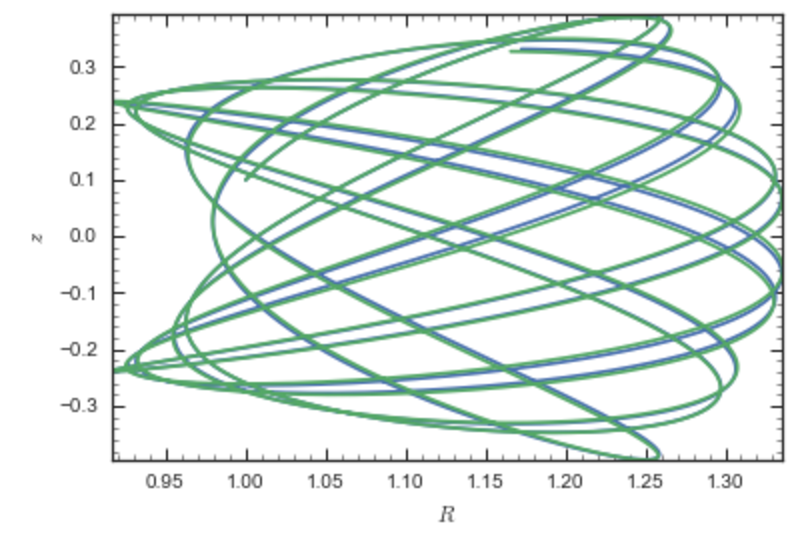
Near the end of the orbit integration, the slight differences between the original potential and the basis-expansion version cause the two orbits to deviate from each other.
If you want to know the basis-function coefficients, you can compute them
using the scf_compute_coeffs_spherical (for
spherically-symmetric density distribution),
scf_compute_coeffs_axi (for
axisymmetric densities), and scf_compute_coeffs (for the general case). The coefficients
obtained from these functions can be directly fed into the
SCFPotential initialization. The basis-function
expansion scale parameter a needs to be passed to both
the scf_compute_coeffs_XX functions and for the SCFPotential
itself. Make sure that you use the same a! Note that the general
functions are quite slow. Equivalent functions for computing the
coefficients based on an N-body snapshot are also available:
scf_compute_coeffs_spherical_nbody, scf_compute_coeffs_axi_nbody, and scf_compute_coeffs_nbody. Note that all of these functions expect a to
be in internal units. The simplest example of computing coefficients
is that of the Hernquist potential, which is the
lowest-order basis function. When we compute the first ten radial
coefficients for this density we obtain that only the lowest-order
coefficient is non-zero
>>> from galpy.potential import HernquistPotential
>>> from galpy.potential import scf_compute_coeffs_spherical
>>> hp= HernquistPotential(amp=1.,a=2.)
>>> Acos, Asin= scf_compute_coeffs_spherical(hp.dens,10,a=2.)
>>> print(Acos)
# array([[[  1.00000000e+00]],
#         [[ -2.83370393e-17]],
#         [[  3.31150709e-19]],
#         [[ -6.66748299e-18]],
#         [[  8.19285777e-18]],
#         [[ -4.26730651e-19]],
#         [[ -7.16849567e-19]],
#         [[  1.52355608e-18]],
#         [[ -2.24030288e-18]],
#         [[ -5.24936820e-19]]])
To then initialize an SCFPotential from these coefficients, do
>>> sp= SCFPotential(Acos=Acos,Asin=Asin,a=2.)
To use the SCF method for disky potentials, we use the trick from Kuijken & Dubinski (1995). This trick works by approximating the disk density as \(\rho_{\mathrm{disk}}(R,\phi,z) \approx \sum_i \Sigma_i(R)\,h_i(z)\), with \(h_i(z) = \mathrm{d}^2 H(z) / \mathrm{d} z^2\) and searching for solutions of the form
\[\Phi(R,\phi,z = \Phi_{\mathrm{ME}}(R,\phi,z) + 4\pi G\sum_i \Sigma_i(r)\,H_i(z)\,,\]
where \(r\) is the spherical radius \(r^2 = R^2+z^2\). The density which gives rise to \(\Phi_{\mathrm{ME}}(R,\phi,z)\) is not strongly confined to a plane when \(\rho_{\mathrm{disk}}(R,\phi,z) \approx \sum_i \Sigma_i(R)\,h_i(z)\) and can be obtained using the SCF basis-function-expansion technique discussed above. See the documentation of the DiskSCFPotential class for more details on this procedure.
As an example, consider a double-exponential disk, which we can
compare to the DoubleExponentialDiskPotential implementation
>>> from galpy import potential
>>> dp= potential.DoubleExponentialDiskPotential(amp=13.5,hr=1./3.,hz=1./27.)
and then setup the DiskSCFPotential approximation to this as
>>> dscfp= potential.DiskSCFPotential(dens=lambda R,z: dp.dens(R,z),
                                      Sigma={'type':'exp','h':1./3.,'amp':1.},
                                      hz={'type':'exp','h':1./27.},
                                      a=1.,N=10,L=10)
The dens= keyword specifies the target density, while the
Sigma= and hz= inputs specify the approximation functions
\(\Sigma_i(R)\) and \(h_i(z)\). These are specified as
dictionaries here for a few pre-defined approximation functions, but
general functions are supported as well. Care should be taken that the
dens= input density and the approximation functions have the same
normalization. We can compare the density along the R=10 z line as
>>> xs= numpy.linspace(0.3,2.,1001)
>>> semilogy(xs,dp.dens(xs,xs/10.))
>>> semilogy(xs,dscfp.dens(xs,xs/10.))
which gives
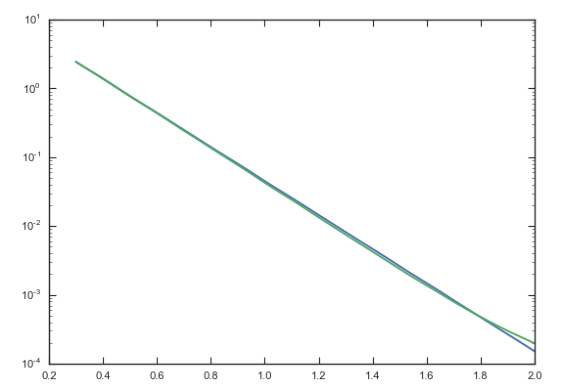
The agreement is good out to 5 scale lengths and scale heights and then starts to degrade. We can also integrate orbits and compare them
>>> from galpy.orbit import Orbit
>>> o= Orbit([1.,0.1,0.9,0.,0.1,0.])
>>> ts= numpy.linspace(0.,100.,10001)
>>> o.integrate(ts,dp)
>>> o.plot()
>>> o.integrate(ts,dscfp)
>>> o.plot(overplot=True)
which gives

The orbits diverge slightly because the potentials are not quite the
same, but have very similar properties otherwise (peri- and
apogalacticons, eccentricity, …). By increasing the order of the SCF
approximation, the potential can be gotten closer to the target
density. Note that orbit integration in the DiskSCFPotential is
much faster than that of the DoubleExponentialDisk potential
>>> %%timeit
>>> o.integrate(ts,dp)
# 4.53 s ± 25.4 ms per loop (mean ± std. dev. of 7 runs, 1 loop each)
and
>>> %%timeit
o.integrate(ts,dscfp)
# 57.2 ms ± 99.6 µs per loop (mean ± std. dev. of 7 runs, 10 loops each)
The SCFPotential and DiskSCFPotential can be used wherever general potentials can be used in galpy.
The potential of N-body simulations
galpy can setup and work with the frozen potential of an N-body
simulation. This allows us to study the properties of such potentials
in the same way as other potentials in galpy. We can also
investigate the properties of orbits in these potentials and calculate
action-angle coordinates, using the galpy framework. Currently,
this functionality is limited to axisymmetrized versions of the N-body
snapshots, although this capability could be somewhat
straightforwardly expanded to full triaxial potentials. The use of
this functionality requires pynbody to be installed; the potential
of any snapshot that can be loaded with pynbody can be used within
galpy.
As a first, simple example of this we look at the potential of a
single simulation particle, which should correspond to galpy’s
KeplerPotential. We can create such a single-particle snapshot
using pynbody by doing
>>> import pynbody
>>> s= pynbody.new(star=1)
>>> s['mass']= 1.
>>> s['eps']= 0.
and we get the potential of this snapshot in galpy by doing
>>> from galpy.potential import SnapshotRZPotential
>>> sp= SnapshotRZPotential(s,num_threads=1)
With these definitions, this snapshot potential should be the same as
KeplerPotential with an amplitude of one, which we can test as
follows
>>> from galpy.potential import KeplerPotential
>>> kp= KeplerPotential(amp=1.)
>>> print(sp(1.1,0.),kp(1.1,0.),sp(1.1,0.)-kp(1.1,0.))
# (-0.90909090909090906, -0.9090909090909091, 0.0)
>>> print(sp.Rforce(1.1,0.),kp.Rforce(1.1,0.),sp.Rforce(1.1,0.)-kp.Rforce(1.1,0.))
# (-0.82644628099173545, -0.8264462809917353, -1.1102230246251565e-16)
SnapshotRZPotential instances can be used wherever other galpy
potentials can be used (note that the second derivatives have not been
implemented, such that functions depending on those will not
work). For example, we can plot the rotation curve
>>> sp.plotRotcurve()
Because evaluating the potential and forces of a snapshot is
computationally expensive, most useful applications of frozen N-body
potentials employ interpolated versions of the snapshot
potential. These can be setup in galpy using an
InterpSnapshotRZPotential class that is a subclass of the
interpRZPotential described above and that can be used in the same
manner. To illustrate its use we will make use of one of pynbody’s
example snapshots, g15784. This snapshot is used here
to illustrate pynbody’s use. Please follow the instructions there
on how to download this snapshot.
Once you have downloaded the pynbody testdata, we can load this
snapshot using
>>> s = pynbody.load('testdata/g15784.lr.01024.gz')
(please adjust the path according to where you downloaded the
pynbody testdata). We get the main galaxy in this snapshot, center
the simulation on it, and align the galaxy face-on using
>>> h = s.halos()
>>> h1 = h[1]
>>> pynbody.analysis.halo.center(h1,mode='hyb')
>>> pynbody.analysis.angmom.faceon(h1, cen=(0,0,0),mode='ssc')
we also convert the simulation to physical units, but set G=1 by doing the following
>>> s.physical_units()
>>> from galpy.util.conversion import _G
>>> g= pynbody.array.SimArray(_G/1000.)
>>> g.units= 'kpc Msol**-1 km**2 s**-2 G**-1'
>>> s._arrays['mass']= s._arrays['mass']*g
We can now load an interpolated version of this snapshot’s potential
into galpy using
>>> from galpy.potential import InterpSnapshotRZPotential
>>> spi= InterpSnapshotRZPotential(h1,rgrid=(numpy.log(0.01),numpy.log(20.),101),logR=True,zgrid=(0.,10.,101),interpPot=True,zsym=True)
where we further assume that the potential is symmetric around the
mid-plane (z=0). This instantiation will take about ten to fiteen
minutes. This potential instance has physical units (and thus the
rgrid= and zgrid= inputs are given in kpc if the simulation’s
distance unit is kpc). For example, if we ask for the rotation curve,
we get the following:
>>> spi.plotRotcurve(Rrange=[0.01,19.9],xlabel=r'$R\,(\mathrm{kpc})$',ylabel=r'$v_c(R)\,(\mathrm{km\,s}^{-1})$')
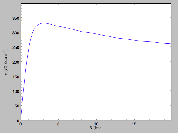
This can be compared to the rotation curve calculated by pynbody,
see here.
Because galpy works best in a system of natural units as
explained in Units in galpy, we will convert this
instance to natural units using the circular velocity at R=10 kpc,
which is
>>> spi.vcirc(10.)
# 294.62723076942245
To convert to natural units we do
>>> spi.normalize(R0=10.)
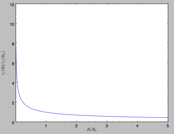
We can then again plot the rotation curve, keeping in mind that the distance unit is now \(R_0\)
>>> spi.plotRotcurve(Rrange=[0.01,1.99])
which gives
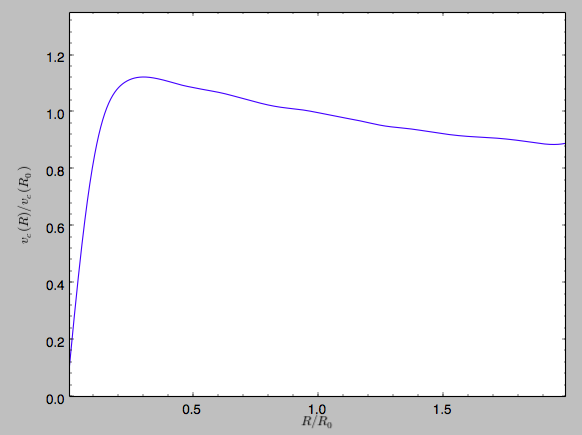
in particular
>>> spi.vcirc(1.)
# 1.0000000000000002
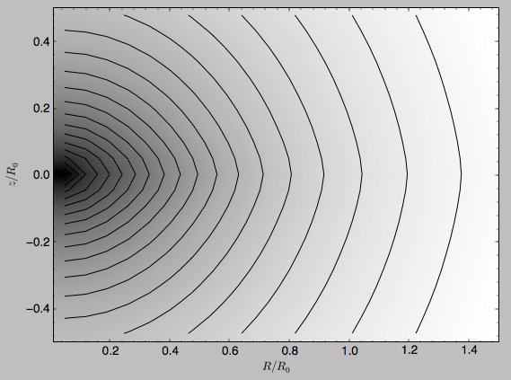
We can also plot the potential
>>> spi.plot(rmin=0.01,rmax=1.9,nrs=51,zmin=-0.99,zmax=0.99,nzs=51)
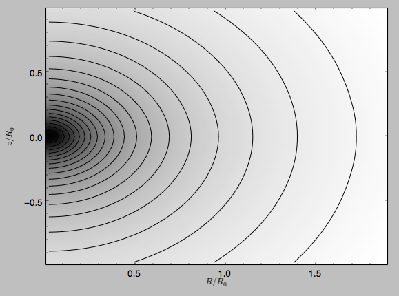
Clearly, this simulation’s potential is quite spherical, which is confirmed by looking at the flattening
>>> spi.flattening(1.,0.1)
# 0.86675711023391921
>>> spi.flattening(1.5,0.1)
# 0.94442750306256895
The epicyle and vertical frequencies can also be interpolated by
setting the interpepifreq=True or interpverticalfreq=True
keywords when instantiating the InterpSnapshotRZPotential object.
Conversion to NEMO potentials
NEMO is a set of tools for
studying stellar dynamics. Some of its functionality overlaps with
that of galpy, but many of its programs are very complementary to
galpy. In particular, it has the ability to perform N-body
simulations with a variety of poisson solvers, which is currently not
supported by galpy (and likely will never be directly
supported). To encourage interaction between galpy and NEMO it
is quite useful to be able to convert potentials between these two
frameworks, which is not completely trivial. In particular, NEMO
contains Walter Dehnen’s fast collisionless gyrfalcON code (see
2000ApJ…536L..39D and
2002JCoPh.179…27D) and the
discussion here focuses on how to run N-body simulations using
external potentials defined in galpy.
Some galpy potential instances support the functions
nemo_accname and nemo_accpars that return the name of the
NEMO potential corresponding to this galpy Potential and its
parameters in NEMO units. These functions assume that you use NEMO
with WD_units, that is, positions are specified in kpc, velocities in
kpc/Gyr, times in Gyr, and G=1. For the Miyamoto-Nagai potential
above, you can get its name in the NEMO framework as
>>> mp.nemo_accname()
# 'MiyamotoNagai'
and its parameters as
>>> mp.nemo_accpars(220.,8.)
# '0,592617.11132,4.0,0.3'
assuming that we scale velocities by vo=220 km/s and positions by
ro=8 kpc in galpy. These two strings can then be given to the
gyrfalcON accname= and accpars= keywords.
We can do the same for lists of potentials. For example, for
MWPotential2014 we do
>>> from galpy.potential import nemo_accname, nemo_accpars
>>> nemo_accname(MWPotential2014)
# 'PowSphwCut+MiyamotoNagai+NFW'
>>> nemo_accpars(MWPotential2014,220.,8.)
# '0,1001.79126907,1.8,1.9#0,306770.418682,3.0,0.28#0,16.0,162.958241887'
Therefore, these are the accname= and accpars= that one needs
to provide to gyrfalcON to run a simulation in
MWPotential2014.
Note that the NEMO potential PowSphwCut is not a standard
NEMO potential. This potential can be found in the nemo/ directory of
the galpy source code; this directory also contains a Makefile that
can be used to compile the extra NEMO potential and install it in
the correct NEMO directory (this requires one to have NEMO
running, i.e., having sourced nemo_start).
You can use the PowSphwCut.cc file in the nemo/ directory as a
template for adding additional potentials in galpy to the NEMO
framework. To figure out how to convert the normalized galpy
potential to an amplitude when scaling to physical coordinates (like
kpc and kpc/Gyr), one needs to look at the scaling of the radial force
with R. For example, from the definition of MiyamotoNagaiPotential, we
see that the radial force scales as \(R^{-2}\). For a general
scaling \(R^{-\alpha}\), the amplitude will scale as
\(V_0^2\,R_0^{\alpha-1}\) with the velocity \(V_0\) and
position \(R_0\) of the v=1 at R=1
normalization. Therefore, for the MiyamotoNagaiPotential, the physical
amplitude scales as \(V_0^2\,R_0\). For the
LogarithmicHaloPotential, the radial force scales as \(R^{-1}\),
so the amplitude scales as \(V_0^2\).
Currently, only the MiyamotoNagaiPotential, NFWPotential,
PowerSphericalPotentialwCutoff, HernquistPotential,
PlummerPotential, MN3ExponentialDiskPotential, and the
LogarithmicHaloPotential have this NEMO support. Combinations of
all but the LogarithmicHaloPotential are allowed in general (e.g.,
MWPotential2014); they can also be combined with spherical
LogarithmicHaloPotentials. Because of the definition of the
logarithmic potential in NEMO, it cannot be flattened in z, so to
use a flattened logarithmic potential, one has to flip y and z
between galpy and NEMO (one can flatten in y).
Conversion to AMUSE potentials
AMUSE is a Python software framework for astrophysical simulations, in which existing codes from different domains, such as stellar dynamics, stellar evolution, hydrodynamics and radiative transfer can be easily coupled. AMUSE allows you to run N-body simulations that include a wide range of physics (gravity, stellar evolution, hydrodynamics, radiative transfer) with a large variety of numerical codes (collisionless, collisional, etc.).
The galpy.potential.to_amuse function allows you to create an
AMUSE representation of any galpy potential. This is useful, for
instance, if you want to run a simulation of a stellar cluster in an
external gravitational field, because galpy has wide support for
representing external gravitational fields. Creating the AMUSE
representation is as simple as (for MWPotential2014):
>>> from galpy.potential import to_amuse, MWPotential2014
>>> mwp_amuse= to_amuse(MWPotential2014)
>>> print(mwp_amuse)
# <galpy.potential.amuse.galpy_profile object at 0x7f6b366d13c8>
Schematically, this potential can then be used in AMUSE as
>>> gravity = bridge.Bridge(use_threading=False)
>>> gravity.add_system(cluster_code, (mwp_amuse,))
>>> gravity.add_system(mwp_amuse,)
where cluster_code is a code to perform the N-body integration of
a system (e.g., a BHTree in AMUSE). A fuller example is given below.
AMUSE uses physical units when interacting with the galpy potential
and it is therefore necessary to make sure that the correct physical
units are used. The to_amuse function takes the galpy unit
conversion parameters ro= and vo= as keyword parameters to
perform the conversion between internal galpy units and physical
units; if these are not explicitly set, to_amuse attempts to set
them automatically using the potential that you input using the
galpy.util.conversion.get_physical function.
Another difference between galpy and AMUSE is that in AMUSE
integration times can only be positive and they have to increase in
time. to_amuse takes as input the t= and tgalpy= keywords
that specify (a) the initial time in AMUSE and (b) the initial time in
galpy that this time corresponds to. Typically these will be the
same (and equal to zero), but if you want to run a simulation where
the initial time in galpy is negative it is useful to give them
different values. The time inputs can be either given in galpy
internal units or using AMUSE’s units. Similarly, to integrate
backwards in time in AMUSE, to_amuse has a keyword reverse=
(default: False) that reverses the time direction given to the
galpy potential; reverse=True does this (note that you also
have to flip the velocities to actually go backwards).
A full example of setting up a Plummer-sphere cluster and evolving its
N-body dynamics using an AMUSE BHTree in the external
MWPotential2014 potential is:
>>> from amuse.lab import *
>>> from amuse.couple import bridge
>>> from amuse.datamodel import Particles
>>> from galpy.potential import to_amuse, MWPotential2014
>>> from galpy.util import plot as galpy_plot
>>>
>>> # Convert galpy MWPotential2014 to AMUSE representation
>>> mwp_amuse= to_amuse(MWPotential2014)
>>>
>>> # Set initial cluster parameters
>>> N= 1000
>>> Mcluster= 1000. | units.MSun
>>> Rcluster= 10. | units.parsec
>>> Rinit= [10.,0.,0.] | units.kpc
>>> Vinit= [0.,220.,0.] | units.km/units.s
>>> # Setup star cluster simulation
>>> tend= 100.0 | units.Myr
>>> dtout= 5.0 | units.Myr
>>> dt= 1.0 | units.Myr
>>>
>>> def setup_cluster(N,Mcluster,Rcluster,Rinit,Vinit):
>>> converter= nbody_system.nbody_to_si(Mcluster,Rcluster)
>>> stars= new_plummer_sphere(N,converter)
>>> stars.x+= Rinit[0]
>>> stars.y+= Rinit[1]
>>> stars.z+= Rinit[2]
>>> stars.vx+= Vinit[0]
>>> stars.vy+= Vinit[1]
>>> stars.vz+= Vinit[2]
>>> return stars,converter
>>>
>>> # Setup cluster
>>> stars,converter= setup_cluster(N,Mcluster,Rcluster,Rinit,Vinit)
>>> cluster_code= BHTree(converter,number_of_workers=1) #Change number of workers depending no. of CPUs
>>> cluster_code.parameters.epsilon_squared= (3. | units.parsec)**2
>>> cluster_code.parameters.opening_angle= 0.6
>>> cluster_code.parameters.timestep= dt
>>> cluster_code.particles.add_particles(stars)
>>>
>>> # Setup channels between stars particle dataset and the cluster code
>>> channel_from_stars_to_cluster_code= stars.new_channel_to(cluster_code.particles,
>>> attributes=["mass", "x", "y", "z", "vx", "vy", "vz"])
>>> channel_from_cluster_code_to_stars= cluster_code.particles.new_channel_to(stars,
>>> attributes=["mass", "x", "y", "z", "vx", "vy", "vz"])
>>>
>>> # Setup gravity bridge
>>> gravity= bridge.Bridge(use_threading=False)
>>> # Stars in cluster_code depend on gravity from external potential mwp_amuse (i.e., MWPotential2014)
>>> gravity.add_system(cluster_code, (mwp_amuse,))
>>> # External potential mwp_amuse still needs to be added to system so it evolves with time
>>> gravity.add_system(mwp_amuse,)
>>> # Set how often to update external potential
>>> gravity.timestep= cluster_code.parameters.timestep/2.
>>> # Evolve
>>> time= 0.0 | tend.unit
>>> while time<tend:
>>> gravity.evolve_model(time+dt)
>>> # If you want to output or analyze the simulation, you need to copy
>>> # stars from cluster_code
>>> #channel_from_cluster_code_to_stars.copy()
>>>
>>> # If you edited the stars particle set, for example to remove stars from the
>>> # array because they have been kicked far from the cluster, you need to
>>> # copy the array back to cluster_code:
>>> #channel_from_stars_to_cluster_code.copy()
>>>
>>> # Update time
>>> time= gravity.model_time
>>>
>>> channel_from_cluster_code_to_stars.copy()
>>> gravity.stop()
>>>
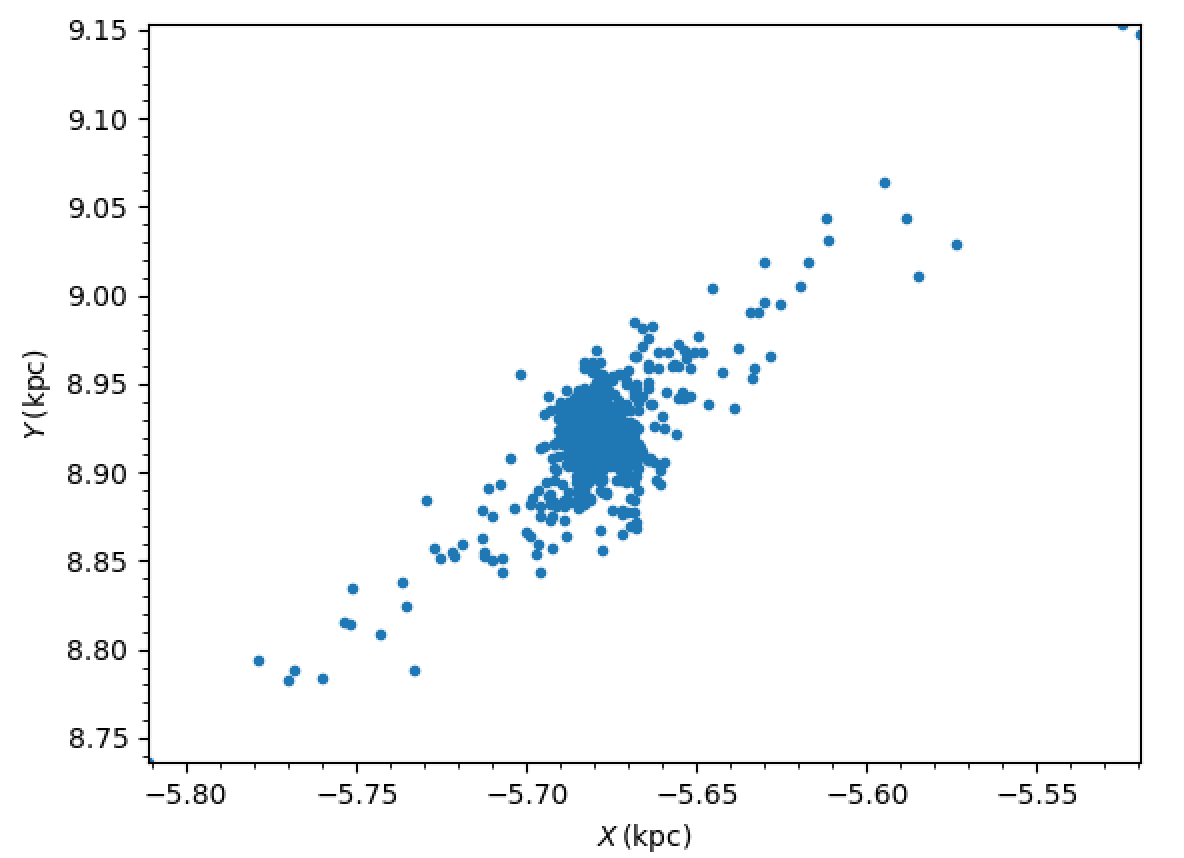
>>> galpy_plot.plot(stars.x.value_in(units.kpc),stars.y.value_in(units.kpc),'.',
>>> xlabel=r'$X\,(\mathrm{kpc})$',ylabel=r'$Y\,(\mathrm{kpc})$')
After about 30 seconds, you should get a plot like the following, which shows a cluster in the first stages of disruption:
Dissipative forces
While almost all of the forces that you can use in galpy derive
from a potential (that is, the force is the gradient of a scalar
function, the potential, meaning that the forces are conservative),
galpy also supports dissipative forces. Dissipative forces all
inherit from the DissipativeForce class and they are required to
take the velocity v=[vR,vT,vZ] in cylindrical coordinates as an
argument to the force in addition to the standard
(R,z,phi=0,t=0). The set of functions evaluateXforces (with
X=R,z,r,phi,etc.) will evaluate the force due to Potential
instances, DissipativeForce instances, or lists of combinations of
these two.
Currently, the dissipative forces implemented in galpy include
ChandrasekharDynamicalFrictionForce, an
implementation of the classic Chandrasekhar dynamical-friction
formula, with recent tweaks to better represent the results from
N-body simulations, and NonInertialFrameForce,
the fictitious forces of a non-inertial reference frame.
Warning
Dissipative forces can currently only be used for 3D orbits in galpy. The code should throw an error when they are used for 2D orbits.
Warning
While we call them ‘dissipative’, what is really meant is that the force depends on the velocity, whether the force is really dissipative or not.
Adding potentials to the galpy framework
Potentials in galpy can be used in many places such as orbit
integration, distribution functions, or the calculation of
action-angle variables, and in most cases any instance of a potential
class that inherits from the general Potential class (or a list of
such instances) can be given. For example, all orbit integration
routines work with any list of instances of the general Potential
class. Adding new potentials to galpy therefore allows them to be used
everywhere in galpy where general Potential instances can be
used. Adding a new class of potentials to galpy consists of the
following series of steps (for steps to add a new wrapper potential,
also see the next section):
- Implement the new potential in a class that inherits from
galpy.potential.Potential(velocity-dependent forces should inherit fromgalpy.potential.DissipativeForceinstead; see below for a brief discussion on differences in implementing such forces). The new class should have an__init__method that sets up the necessary parameters for the class. An amplitude parameteramp=and two units parametersro=andvo=should be taken as an argument for this class and before performing any other setup, thegalpy.potential.Potential.__init__(self,amp=amp,ro=ro,vo=vo,amp_units=)method should be called to setup the amplitude and the system of units; theamp_units=keyword specifies the physical units of the amplitude parameter (e.g.,amp_units='velocity2'when the units of the amplitude are velocity-squared) To add support for normalizing the potential to standard galpy units, one can call thegalpy.potential.Potential.normalizefunction at the end of the __init__ function.
The new potential class should implement some of the following functions:
_evaluate(self,R,z,phi=0,t=0)which evaluates the potential itself (without the amp factor, which is added in the__call__method of the general Potential class)._Rforce(self,R,z,phi=0.,t=0.)which evaluates the radial force in cylindrical coordinates (-d potential / d R)._zforce(self,R,z,phi=0.,t=0.)which evaluates the vertical force in cylindrical coordinates (-d potential / d z)._R2deriv(self,R,z,phi=0.,t=0.)which evaluates the second (cylindrical) radial derivative of the potential (d^2 potential / d R^2)._z2deriv(self,R,z,phi=0.,t=0.)which evaluates the second (cylindrical) vertical derivative of the potential (d^2 potential / d z^2)._Rzderiv(self,R,z,phi=0.,t=0.)which evaluates the mixed (cylindrical) radial and vertical derivative of the potential (d^2 potential / d R d z)._dens(self,R,z,phi=0.,t=0.)which evaluates the density. If not given, the density is computed using the Poisson equation from the first and second derivatives of the potential (if all are implemented)._mass(self,R,z=0.,t=0.)which evaluates the mass. For spherical potentials this should give the mass enclosed within the spherical radius; for axisymmetric potentials this should return the mass up toRand between-ZandZ. If not given, the mass is computed by integrating the density (if it is implemented or can be calculated from the Poisson equation)._phitorque(self,R,z,phi=0.,t=0.): the azimuthal torque in cylindrical coordinates (assumed zero if not implemented)._phi2deriv(self,R,z,phi=0.,t=0.): the second azimuthal derivative of the potential in cylindrical coordinates (d^2 potential / d phi^2; assumed zero if not given)._Rphideriv(self,R,z,phi=0.,t=0.): the mixed radial and azimuthal derivative of the potential in cylindrical coordinates (d^2 potential / d R d phi; assumed zero if not given).OmegaP(self): returns the pattern speed for potentials with a pattern speed (used to compute the Jacobi integral for orbits).If you want to be able to calculate the concentration for a potential, you also have to set
self._scaleto a scale parameter for your potential.The code for
galpy.potential.MiyamotoNagaiPotentialgives a good template to follow for 3D axisymmetric potentials. Similarly, the code forgalpy.potential.CosmphiDiskPotentialprovides a good template for 2D, non-axisymmetric potentials.During development or if some of the forces or second derivatives are too tedious to implement, it is possible to numerically compute any non-implemented forces and second derivatives by inheriting from the NumericalPotentialDerivativesMixin class. Thus, a functioning potential can be implemented by simply implementing the
_evaluatefunction and adding all forces and second derivatives using theNumericalPotentialDerivativesMixin.After this step, the new potential will work in any part of galpy that uses pure python potentials. To get the potential to work with the C implementations of orbit integration or action-angle calculations, the potential also has to be implemented in C and the potential has to be passed from python to C (see below).
The
__init__method should be written in such a way that a relevant object can be initialized usingClassname()(i.e., there have to be reasonable defaults given for all parameters, including the amplitude); doing this allows the nose tests for potentials to automatically check that your Potential’s potential function, force functions, second derivatives, and density (through the Poisson equation) are correctly implemented (if they are implemented). The continuous-integration platform that builds the galpy codebase upon code pushes will then automatically test all of this, streamlining push requests of new potentials.A few atrributes need to be set depending on the potential:
hasC=Truefor potentials for which the forces and potential are implemented in C (see below);self.hasC_dxdv=Truefor potentials for which the (planar) second derivatives are implemented in C;self.hasC_dens=Truefor potentials for which the density is implemented in C as well (necessary for them to work with dynamical friction in C);self.isNonAxi=Truefor non-axisymmetric potentials.
- To add a C implementation of the potential, implement it in a .c file under
potential/potential_c_ext. Look atpotential/potential_c_ext/LogarithmicHaloPotential.cfor the right format for 3D, axisymmetric potentials, or atpotential/potential_c_ext/LopsidedDiskPotential.cfor 2D, non-axisymmetric potentials.
For orbit integration, the functions such as:
- double LogarithmicHaloPotentialRforce(double R,double Z, double phi,double t,struct potentialArg * potentialArgs)
- double LogarithmicHaloPotentialzforce(double R,double Z, double phi,double t,struct potentialArg * potentialArgs)
are most important. For some of the action-angle calculations
- double LogarithmicHaloPotentialEval(double R,double Z, double phi,double t,struct potentialArg * potentialArgs)
is most important (i.e., for those algorithms that evaluate the potential). If you want your potential to be able to be used as the density for the ChandrasekharDynamicalFrictionForce implementation in C, you need to implement the density in C as well
- double LogarithmicHaloPotentialDens(double R,double Z, double phi,double t,struct potentialArg * potentialArgs)
The arguments of the potential are passed in a
potentialArgsstructure that containsargs, which are the arguments that should be unpacked. Again, looking at some example code will make this clear. ThepotentialArgsstructure is defined inpotential/potential_c_ext/galpy_potentials.h.
3. Add the potential’s function declarations to
potential/potential_c_ext/galpy_potentials.h
4. (4. and 5. for planar orbit integration) Edit the code under
orbit/orbit_c_ext/integratePlanarOrbit.c to set up your new
potential (in the parse_leapFuncArgs function).
5. Edit the code in orbit/integratePlanarOrbit.py to set up your
new potential (in the _parse_pot function).
6. Edit the code under orbit/orbit_c_ext/integrateFullOrbit.c to
set up your new potential (in the parse_leapFuncArgs_Full function).
7. Edit the code in orbit/integrateFullOrbit.py to set up your
new potential (in the _parse_pot function).
8. Finally, add self.hasC= True to the initialization of the
potential in question (after the initialization of the super class, or
otherwise it will be undone). If you have implemented the necessary
second derivatives for integrating phase-space volumes, also add
self.hasC_dxdv=True. If you have implemented the density in C, set
self.hasC_dens=True.
After following the relevant steps, the new potential class can be used in any galpy context in which C is used to speed up computations.
Velocity-dependent forces (e.g.,
ChandrasekharDynamicalFrictionForce) should inherit from galpy.potential.DissipativeForce instead of from galpy.potential.Potential. Because such forces are not conservative, you only need to implement the forces themselves, in the same way as for a regular Potential. For dissipative forces, the force-evaluation functions (Rforce, etc.) need to take the velocity in cylindrical coordinates as a keyword argument: v=[vR,vT,vZ]. Implementing dissipative forces in C is similar: you only need to implement the forces themselves and the forces should take the velocity in cylindrical coordinates as an additional input, e.g.,
- double ChandrasekharDynamicalFrictionForceRforce(double R,double z, double phi,double t,struct potentialArg * potentialArgs,double vR,double vT,double vz)
Adding wrapper potentials to the galpy framework
Wrappers all inherit from the general WrapperPotential or
planarWrapperPotential classes (which themselves inherit from the
Potential and planarPotential classes and therefore all
wrappers are Potentials or planarPotentials). Depending on the
complexity of the wrapper, wrappers can be implemented much more
economically in Python than new Potential instances as described
above.
To add a Python implementation of a new wrapper, classes need to
inherit from parentWrapperPotential, take the potentials to be
wrapped as a pot= (a Potential, planarPotential, or a list
thereof; automatically assigned to self._pot) input to
__init__, and implement the
_wrap(self,attribute,*args,**kwargs) function. This function
modifies the Potential functions _evaluate, _Rforce, etc. (all
of those listed above), with attribute the
function that is being modified. Inheriting from
parentWrapperPotential gives the class access to the
self._wrap_pot_func(attribute) function which returns the relevant
function for each attribute. For example,
self._wrap_pot_func('_evaluate') returns the
evaluatePotentials function that can then be called as
self._wrap_pot_func('_evaluate')(self._pot,R,Z,phi=phi,t=t) to
evaluate the potentials being wrapped. By making use of
self._wrap_pot_func, wrapper potentials can be implemented in just
a few lines. Your __init__ function should only initialize
things in your wrapper; there is no need to manually assign
self._pot or to call the superclass’ __init__ (all
automatically done for you!).
To correctly work with both 3D and 2D potentials, inputs to _wrap
need to be specified as *args,**kwargs: grab the values you need
for R,z,phi,t from these as R=args[0], z=0 if len(args) == 1
else args[1], phi=kwargs.get('phi',0.), t=kwargs.get('t',0.), where
the complicated expression for z is to correctly deal with both 3D and
2D potentials (of course, if your wrapper depends on z, it probably
doesn’t make much sense to apply it to a 2D planarPotential; you could
check the dimensionality of self._pot in your wrapper’s
__init__ function with from galpy.potential.Potential._dim
and raise an error if it is not 3 in this case). Wrapping a 2D
potential automatically results in a wrapper that is a subclass of
planarPotential rather than Potential; this is done by the
setup in parentWrapperPotential and hidden from the user. For
wrappers of planar Potentials, self._wrap_pot_func(attribute) will
return the evaluateplanarPotentials etc. functions instead, but
this is again hidden from the user if you implement the _wrap
function as explained above.
As an example, for the DehnenSmoothWrapperPotential, the _wrap
function is
def _wrap(self,attribute,*args,**kwargs):
    return self._smooth(kwargs.get('t',0.))\
            *self._wrap_pot_func(attribute)(self._pot,*args,**kwargs)
where smooth(t) returns the smoothing function of the
amplitude. When any of the basic Potential functions are called
(_evaluate, _Rforce, etc.), _wrap gets called by the
superclass WrapperPotential, and the _wrap function returns
the corresponding function for the wrapped potentials with the
amplitude modified by smooth(t). Therefore, one does not need to
implement each of the _evaluate, _Rforce, etc. functions like
for regular potential. The rest of the
DehnenSmoothWrapperPotential is essentially (slightly simplified
in non-crucial aspects)
def __init__(self,amp=1.,pot=None,tform=-4.,tsteady=None,ro=None,vo=None):
    # Note: (i) don't assign self._pot and (ii) don't run super.__init__
    self._tform= tform
    if tsteady is None:
        self._tsteady= self._tform/2.
    else:
        self._tsteady= self._tform+tsteady
    self.hasC= True
    self.hasC_dxdv= True

def _smooth(self,t):
    #Calculate relevant time
    if t < self._tform:
        smooth= 0.
    elif t < self._tsteady:
        deltat= t-self._tform
        xi= 2.*deltat/(self._tsteady-self._tform)-1.
        smooth= (3./16.*xi**5.-5./8*xi**3.+15./16.*xi+.5)
    else: #bar is fully on
        smooth= 1.
    return smooth
The source code for DehnenSmoothWrapperPotential potential may act
as a guide to implementing new wrappers.
C implementations of potential wrappers can also be added in a similar
way as C implementations of regular potentials (all of the steps
listed in the previous section for adding a
potential to C need to be followed). All of the necessary functions
(...Rforce, ...zforce, ..phitorque, etc.) need to be
implemented separately, but by including galpy_potentials.h
calling the relevant functions of the wrapped potentials is easy. Look
at DehnenSmoothWrapperPotential.c for an example that can be
straightforwardly edited for other wrappers.
The glue between Python and C for wrapper potentials needs to glue
both the wrapper and the wrapped potentials. This can be easily
achieved by recursively calling the _parse_pot glue functions in
Python (see the previous section; this needs to be done separately for
each potential currently) and the parse_leapFuncArgs and
parse_leapFuncArgs_Full functions in C (done automatically for all
wrappers). Again, following the example of
DehnenSmoothWrapperPotential.py should allow for a straightforward
implementation of the glue for any new wrappers. Wrapper potentials
should be given negative potential types in the glue to distinguish
them from regular potentials.
Adding dissipative forces to the galpy framework
Dissipative forces are implemented in much the same way as forces that
derive from potentials. Rather than inheriting from
galpy.potential.Potential, dissipative forces inherit from
galpy.potential.DissipativeForce. The procedure for implementing a
new class of dissipative force is therefore very similar to that for
implementing a new potential. The main differences
are that (a) you only need to implement the forces and (b) the forces
are required to take an extra keyword argument v= that gives the
velocity in cylindrical coordinates (because dissipative forces will
in general depend on the current velocity). Thus, the steps are:
- Implement the new dissipative force in a class that inherits from
galpy.potential.DissipativeForce. The new class should have an__init__method that sets up the necessary parameters for the class. An amplitude parameteramp=and two units parametersro=andvo=should be taken as an argument for this class and before performing any other setup, thegalpy.potential.DissipativeForce.__init__(self,amp=amp,ro=ro,vo=vo,amp_units=)method should be called to setup the amplitude and the system of units; theamp_units=keyword specifies the physical units of the amplitude parameter (e.g.,amp_units='mass'when the units of the amplitude are mass)
The new dissipative-force class should implement the following functions:
_Rforce(self,R,z,phi=0.,t=0.,v=None)which evaluates the radial force in cylindrical coordinates_phitorque(self,R,z,phi=0.,t=0.,v=None)which evaluates the azimuthal force in cylindrical coordinates_zforce(self,R,z,phi=0.,t=0.,v=None)which evaluates the vertical force in cylindrical coordinatesThe code for
galpy.potential.ChandrasekharDynamicalFrictionForcegives a good template to follow.
2. That’s it, as for now there is no support for implementing a C version of dissipative forces.