Potential (galpy.potential)
3D potentials
General instance routines
Use as Potential-instance.method(...)
- __add__
- __mul__
- __call__
- dens
- dvcircdR
- epifreq
- flattening
- LcE
- lindbladR
- mass
- nemo_accname
- nemo_accpars
- omegac
- phitorque
- phizderiv
- phi2deriv
- plot
- plotDensity
- plotEscapecurve
- plotRotcurve
- plotSurfaceDensity
- R2deriv
- r2deriv
- rE
- Rzderiv
- Rforce
- rforce
- rhalf
- rl
- Rphideriv
- rtide
- surfdens
- tdyn
- toPlanar
- toVertical
- ttensor
- turn_physical_off
- turn_physical_on
- vcirc
- verticalfreq
- vesc
- vterm
- z2deriv
- zforce
- zvc
- zvc_range
In addition to these, the NFWPotential also has methods to calculate virial quantities
General 3D potential routines
Use as method(...)
- dvcircdR
- epifreq
- evaluateDensities
- evaluatephitorques
- evaluatePotentials
- evaluatephizderivs
- evaluatephi2derivs
- evaluateRphiderivs
- evaluateR2derivs
- evaluater2derivs
- evaluateRzderivs
- evaluateRforces
- evaluaterforces
- evaluateSurfaceDensities
- evaluatez2derivs
- evaluatezforces
- flatten
- flattening
- LcE
- lindbladR
- mass
- nemo_accname
- nemo_accpars
- omegac
- plotDensities
- plotEscapecurve
- plotPotentials
- plotRotcurve
- plotSurfaceDensities
- rE
- rhalf
- rl
- rtide
- tdyn
- to_amuse
- ttensor
- turn_physical_off
- turn_physical_on
- vcirc
- verticalfreq
- vesc
- vterm
- zvc
- zvc_range
In addition to these, the following methods are available to compute expansion coefficients for the SCFPotential class for a given density
Specific potentials
All of the following potentials can also be modified by the specific WrapperPotentials listed below.
Spherical potentials
Spherical potentials in galpy can be implemented in two ways: a)
directly by inheriting from Potential and implementing the usual
methods (_evaluate, _Rforce, etc.) or b) by inheriting from
the general SphericalPotential class and
implementing the functions _revaluate(self,r,t=0.),
_rforce(self,r,t=0.), _r2deriv(self,r,t=0.), and
_rdens(self,r,t=0.) that evaluate the potential, radial force,
(minus the) radial force derivative, and density as a function of the
(here natural) spherical radius. For adding a C implementation when
using method b), follow similar steps in C (use
interpSphericalPotential as an example to follow). For historical
reasons, most spherical potentials in galpy are directly
implemented (option a above), but for new spherical potentials it is
typically easier to follow option b).
Additional spherical potentials can be obtained by setting the axis ratios equal for the triaxial potentials listed in the section on ellipsoidal triaxial potentials below.
- Arbitrary spherical density potential
- Burkert potential
- Double power-law density spherical potential
- Spherical Cored Dehnen potential
- Spherical Dehnen potential
- Hernquist potential
- Homogeneous sphere potential
- Interpolated spherical potential
- Isochrone potential
- Jaffe potential
- Kepler potential
- NFW potential
- Plummer potential
- Power-law density spherical potential
- Power-law density spherical potential with an exponential cut-off
- Pseudo-isothermal potential
- Spherical Shell Potential
Axisymmetric potentials
Additional axisymmetric potentials can be obtained by setting the x/y axis ratio equal to 1 for the triaxial potentials listed in the section on ellipsoidal triaxial potentials below.
- Arbitrary razor-thin, axisymmetric potential
- Double exponential disk potential
- Flattened Power-law potential
- Interpolated axisymmetric potential
- Interpolated SnapshotRZ potential
- Kuzmin disk potential
- Kuzmin-Kutuzov Staeckel potential
- Logarithmic halo potential
- Miyamoto-Nagai potential
- Three Miyamoto-Nagai disk approximation to an exponential disk
- Razor-thin exponential disk potential
- Ring potential
- Axisymmetrized N-body snapshot potential
Ellipsoidal triaxial potentials
galpy has very general support for implementing triaxial (or the
oblate and prolate special cases) of ellipsoidal potentials through
the general EllipsoidalPotential class. These
potentials have densities that are uniform on ellipsoids, thus only
functions of \(m^2 = x^2 + \frac{y^2}{b^2}+\frac{z^2}{c^2}\). New
potentials of this type can be implemented by inheriting from this
class and implementing the _mdens(self,m), _psi(self,m), and
_mdens_deriv functions for the density, its integral with respect
to \(m^2\), and its derivative with respect to m,
respectively. For adding a C implementation, follow similar steps (use
PerfectEllipsoidPotential as an example to follow).
Note that the Ferrers potential listed below is a potential of this
type, but it is currently not implemented using the
EllipsoidalPotential class. Further note that these potentials can
all be rotated in 3D using the zvec and pa keywords; however,
more general support for the same behavior is available through the
RotateAndTiltWrapperPotential discussed below and the internal
zvec/pa keywords will likely be deprecated in a future
version.
Spiral, bar, other triaxial, and miscellaneous potentials
All galpy potentials can also be made to rotate using the SolidBodyRotationWrapperPotential listed in the section on wrapper potentials below.
General Poisson solvers for disks and halos
Dissipative forces
Fictitious forces in non-inertial frames
Milky-Way-like potentials
galpy contains various simple models for the Milky Way’s
gravitational potential. The recommended model, described in Bovy
(2015), is included as
galpy.potential.MWPotential2014. This potential was fit to a large
variety of data on the Milky Way and thus serves as both a simple and
accurate model for the Milky Way’s potential (see Bovy 2015 for full information on how this
potential was fit). Note that this potential assumes a circular
velocity of 220 km/s at the solar radius at 8 kpc. This potential is
defined as
>>> bp= PowerSphericalPotentialwCutoff(alpha=1.8,rc=1.9/8.,normalize=0.05)
>>> mp= MiyamotoNagaiPotential(a=3./8.,b=0.28/8.,normalize=.6)
>>> np= NFWPotential(a=16/8.,normalize=.35)
>>> MWPotential2014= bp+mp+np
and can thus be used like any list of Potentials. The mass of the
dark-matter halo in MWPotential2014 is on the low side of
estimates of the Milky Way’s halo mass; if you want to adjust it, for
example making it 50% larger, you can simply multiply the halo part of
MWPotential2014 by 1.5 as (this type of multiplication works for
any potential in galpy)
>>> MWPotential2014[2]*= 1.5
If one wants to add the supermassive black hole at the Galactic center, this can be done by
>>> from galpy.potential import KeplerPotential
>>> from galpy.util import conversion
>>> MWPotential2014wBH= MWPotential2014+KeplerPotential(amp=4*10**6./conversion.mass_in_msol(220.,8.))
for a black hole with a mass of \(4\times10^6\,M_{\odot}\). If you want to take into account dynamical friction for, say, an object of mass \(5\times 10^{10}\,M_\odot\) and a half-mass radius of 5 kpc, do
>>> from galpy.potential import ChandrasekharDynamicalFrictionForce
>>> from astropy import units
>>> cdf= ChandrasekharDynamicalFrictionForce(GMs=5.*10.**10.*units.Msun,
                                             rhm=5.*units.kpc,
                                             dens=MWPotential2014)
>>> MWPotential2014wDF= MWPotential2014+cdf
where we have specified the parameters of the dynamical friction with units; alternatively, convert them directly to galpy natural units as
>>> cdf= ChandrasekharDynamicalFrictionForce(GMs=5.*10.**10./conversion.mass_in_msol(220.,8.),
                                             rhm=5./8.,
                                             dens=MWPotential2014)
>>> MWPotential2014wDF= MWPotential2014+cdf
As explained in this section, without this black
hole or dynamical friction, MWPotential2014 can be used with
Dehnen’s gyrfalcON code using accname=PowSphwCut+MiyamotoNagai+NFW
and
accpars=0,1001.79126907,1.8,1.9#0,306770.418682,3.0,0.28#0,16.0,162.958241887.
galpy also contains other models for the Milky Way’s potential
from the literature in the galpy.potential.mwpotentials module
(which also contains MWPotential2014). Currently, these are:
McMillan17: the potential model from McMillan (2017)Irrgang13I: model I from Irrgang et al. (2013), which is an updated version of the classic Allen & Santillan (1991)Irrgang13IIandIrrgang13III: model II and III from Irrgang et al. (2013)Cautun20: the potential model from Cautun et al. (2020)DehnenBinney98I,DehnenBinney98II,DehnenBinney98III, andDehnenBinney98IVfor models 1 through 4 from Dehnen & Binney (1998).
Unlike MWPotential2014, these potentials have physical units
turned on, using as the unit scaling parameters ro and vo the
distance to the Galactic center and the circular velocity at the Sun’s
radius of each potential. These can be obtained using the
galpy.util.conversion.get_physical function, e.g.,
>>> from galpy.potential.mwpotentials import McMillan17
>>> from galpy.util.conversion import get_physical
>>> get_physical(McMillan17)
# {'ro': 8.21, 'vo': 233.1}
This function returns the unit-conversion parameters as a dictionary,
so they can be easily passed to other functions. For example, when
integrating an orbit in these potentials and either initializing the
orbit using observed coordinates or converting the integrated orbit to
observed coordinates, it is important to use the same unit-conversion
parameters (otherwise an error will be raised). For example, to obtain
the orbit of the Sun in the McMillan17 potential, we do
>>> from galpy.orbit import Orbit
>>> o= Orbit(**get_physical(McMillan17))
As an example, we integrate the Sun’s orbit for 10 Gyr in
MWPotential2014, McMillan17 and Irrgang13I
>>> from galpy.potential.mwpotentials import MWPotential2014, McMillan17, Irrgang13I
>>> from galpy.orbit import Orbit
>>> from galpy.util.conversion import get_physical
>>> from astropy import units
>>> times= numpy.linspace(0.,10.,3001)*units.Gyr
>>> o_mwp14= Orbit(ro=8.,vo=220.) # Need to set these by hand
>>> o_mcm17= Orbit(**get_physical(McMillan17))
>>> o_irrI= Orbit(**get_physical(Irrgang13I))
>>> o_mwp14.integrate(times,MWPotential2014)
>>> o_mcm17.integrate(times,McMillan17)
>>> o_irrI.integrate(times,Irrgang13I)
>>> o_mwp14.plot(lw=0.6)
>>> o_mcm17.plot(overplot=True,lw=0.6)
>>> o_irrI.plot(overplot=True,lw=0.6)
which gives
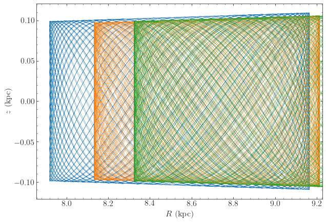
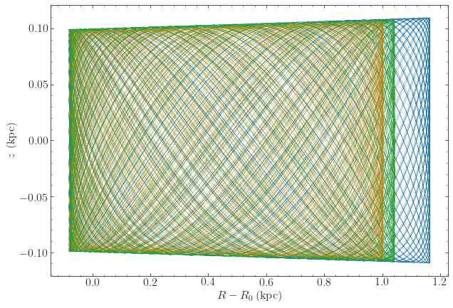
Much of the difference between these orbits is due to the different present Galactocentric radius of the Sun, if we simply plot the difference with respect to the present Galactocentric radius, they agree better
>>> o_mwp14.plot(d1='R-8.',d2='z',lw=0.6,xlabel=r'$R-R_0\,(\mathrm{kpc})$')
>>> o_mcm17.plot(d1='R-{}'.format(get_physical(McMillan17)['ro']),d2='z',overplot=True,lw=0.6)
>>> o_irrI.plot(d1='R-{}'.format(get_physical(Irrgang13I)['ro']),d2='z',overplot=True,lw=0.6)
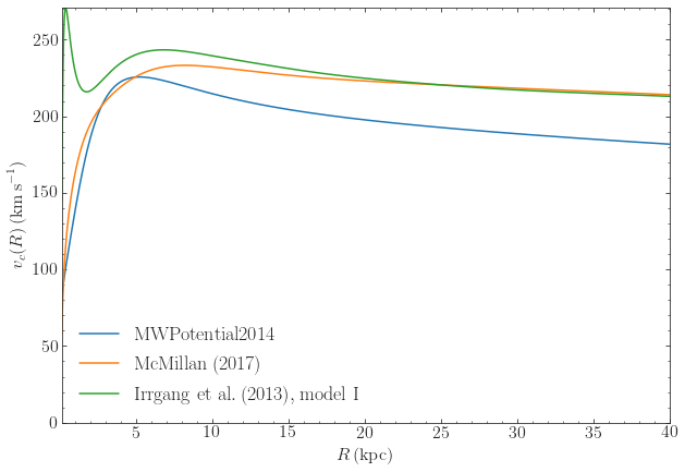
We can also compare the rotation curves of these different models
>>> from galpy.potential import plotRotcurve
>>> plotRotcurve(MWPotential2014,label=r'$\mathrm{MWPotential2014}$',ro=8.,vo=220.) # need to set ro and vo explicitly, because MWPotential2014 has units turned off
>>> plotRotcurve(McMillan17,overplot=True,label=r'$\mathrm{McMillan\, (2017)}$')
>>> plotRotcurve(Irrgang13I,overplot=True,label=r'$\mathrm{Irrgang\ et\ al.\, (2017), model\ I}$')
>>> legend()
An older version galpy.potential.MWPotential of
MWPotential2014 that was not fit to data on the Milky Way is
defined as
>>> mp= MiyamotoNagaiPotential(a=0.5,b=0.0375,normalize=.6)
>>> np= NFWPotential(a=4.5,normalize=.35)
>>> hp= HernquistPotential(a=0.6/8,normalize=0.05)
>>> MWPotential= mp+np+hp
but galpy.potential.MWPotential2014 supersedes
galpy.potential.MWPotential and its use is no longer recommended.
2D potentials
General instance routines
Use as Potential-instance.method(...)
General axisymmetric potential instance routines
Use as Potential-instance.method(...)
General 2D potential routines
Use as method(...)
Specific potentials
All of the 3D potentials above can be used as two-dimensional potentials in the mid-plane.
In addition, a two-dimensional bar potential, two spiral potentials, the Henon & Heiles (1964) potential, and some static non-axisymmetric perturbations are included
1D potentials
General instance routines
Use as Potential-instance.method(...)
General 1D potential routines
Use as method(...)
Specific potentials
One-dimensional potentials can also be derived from 3D axisymmetric potentials as the vertical potential at a certain Galactocentric radius
Potential wrappers
Gravitational potentials in galpy can also be modified using wrappers, for example, to change their amplitude as a function of time. These wrappers can be applied to any galpy potential (although whether they can be used in C depends on whether the wrapper and all of the potentials that it wraps are implemented in C). Multiple wrappers can be applied to the same potential.