This page was generated from a Jupyter notebook. You can download it here.

Fast Orbit Characterization

Orbit integration can be expensive when you only need basic orbital parameters like eccentricity, pericenter, apocenter, or maximum height above the plane. The Staeckel approximation provides a fast alternative that avoids integration entirely. It also allows you to estimate the actions, angles, and frequencies of an orbit.

%matplotlib inline
import numpy
from galpy.orbit import Orbit
from galpy.potential import MWPotential2014
from galpy.actionAngle import estimateDeltaStaeckel
import warnings

warnings.filterwarnings("ignore", category=RuntimeWarning)
warnings.filterwarnings("ignore", category=UserWarning)

Staeckel approximation for a single orbit

Use analytic=True with type='staeckel' to compute orbital parameters without integrating. The Staeckel focal length delta is estimated automatically.

o = Orbit([1.0, 0.1, 1.0, 0.0, 0.1, 0.0])

e_staeckel = o.e(analytic=True, pot=MWPotential2014, type="staeckel")
rap_staeckel = o.rap(analytic=True, pot=MWPotential2014, type="staeckel")
rperi_staeckel = o.rperi(analytic=True, pot=MWPotential2014, type="staeckel")
zmax_staeckel = o.zmax(analytic=True, pot=MWPotential2014, type="staeckel")

print(f"Eccentricity: {e_staeckel:.4f}")
print(f"Apocenter:    {rap_staeckel:.4f}")
print(f"Pericenter:   {rperi_staeckel:.4f}")
print(f"zmax:         {zmax_staeckel:.4f}")

Eccentricity: 0.0749
Apocenter:    1.0845
Pericenter:   0.9333
zmax:         0.0431

Note that type='staeckel' is the default when analytic=True, so you can omit it if you want.

Multiple orbits at once

The Staeckel approximation works efficiently for arrays of orbits.

numpy.random.seed(42)
N = 1000
vxvvs = numpy.column_stack(
    [
        numpy.random.uniform(0.5, 1.5, N),
        numpy.random.normal(0.0, 0.1, N),
        numpy.random.uniform(0.8, 1.2, N),
        numpy.random.normal(0.0, 0.1, N),
        numpy.random.normal(0.0, 0.1, N),
        numpy.random.uniform(0.0, 2 * numpy.pi, N),
    ]
)
os = Orbit(vxvvs)
eccs = os.e(analytic=True, pot=MWPotential2014, type="staeckel")
print(f"Computed {len(eccs)} eccentricities")
print(f"Mean eccentricity: {numpy.mean(eccs):.4f}")
print(f"Std eccentricity:  {numpy.std(eccs):.4f}")

Computed 1000 eccentricities
Mean eccentricity: 0.1338
Std eccentricity:  0.0635

Estimating the Staeckel focal length

The estimateDeltaStaeckel function computes the optimal focal length delta for a given position in a potential. This is done automatically by the orbit methods, but you can also call it directly.

# For a single position
delta = estimateDeltaStaeckel(MWPotential2014, 1.0, 0.1)
print(f"Estimated delta: {delta:.4f}")

# For an array of positions
Rs = numpy.random.uniform(0.5, 1.5, 100)
zs = numpy.random.normal(0.0, 0.1, 100)
deltas = estimateDeltaStaeckel(MWPotential2014, Rs, zs)
print(f"Mean delta: {numpy.mean(deltas):.4f}")

Estimated delta: 0.4033
Mean delta: 0.4502

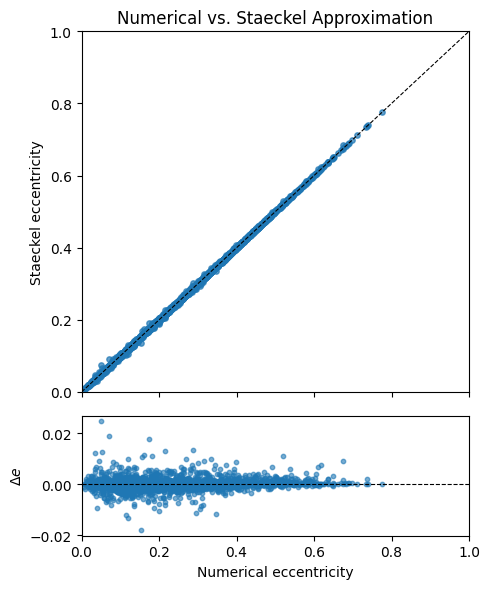
Comparison: numerical vs. Staeckel

Let’s compare orbital parameters computed by orbit integration vs. the Staeckel approximation.

import matplotlib.pyplot as plt

numpy.random.seed(42)
N_cmp = 5000
vxvvs_cmp = numpy.column_stack(
    [
        numpy.random.uniform(0.6, 2.4, N_cmp),
        numpy.random.normal(0.0, 0.28, N_cmp),
        numpy.random.uniform(0.85, 1.15, N_cmp),
        numpy.random.uniform(0.01, 0.2, N_cmp),
        numpy.random.normal(0.0, 0.28, N_cmp),
        numpy.random.uniform(0.0, 2 * numpy.pi, N_cmp),
    ]
)
os_cmp = Orbit(vxvvs_cmp)

# Numerical: integrate then compute
ts = numpy.linspace(0.0, 50.0, 5_000)
os_cmp.integrate(ts, MWPotential2014)
e_num = os_cmp.e()

# Staeckel: no integration needed
e_ana = os_cmp.e(analytic=True, pot=MWPotential2014)

# Two-panel comparison with shared x-axis
fig, (ax_top, ax_bot) = plt.subplots(
    2, 1, sharex=True, figsize=(5, 6), gridspec_kw={"height_ratios": [3, 1]}
)

# Top: direct comparison
ax_top.plot([0, 1], [0, 1], "k--", lw=0.8)
ax_top.scatter(e_num, e_ana, s=15, alpha=0.7)
ax_top.set_ylabel("Staeckel eccentricity")
ax_top.set_title("Numerical vs. Staeckel Approximation")
ax_top.set_xlim(0, 1.0)
ax_top.set_ylim(0, 1.0)

# Bottom: difference
diff = e_ana - e_num
ax_bot.axhline(0.0, color="k", ls="--", lw=0.8)
ax_bot.scatter(e_num, diff, s=10, alpha=0.6)
ax_bot.set_xlabel("Numerical eccentricity")
ax_bot.set_ylabel(r"$\Delta e$")

plt.tight_layout()

Actions, angles, and frequencies

The Staeckel approximation also provides estimates of the actions, angles, and frequencies of an orbit (see Binney 2012). This is discussed in more detail in the Staeckel Approximation tutorial, but we can also compute these quantities when analytic=True:

o = Orbit([1.0, 0.1, 1.0, 0.0, 0.1, 0.0])

jr_staeckel = o.jr(analytic=True, pot=MWPotential2014, type="staeckel")
jz_staeckel = o.jz(analytic=True, pot=MWPotential2014, type="staeckel")

print(f"Radial action: {jr_staeckel:.4f}")
print(f"Vertical action: {jz_staeckel:.4f}")

Radial action: 0.0038
Vertical action: 0.0020

Note that the angular momentum is the third action, so it is exact regardless of the approximation used:

lz = o.Lz()
print(f"Angular momentum: {lz:.4f}")

Angular momentum: 1.0000

We can also return actions with physical units, e.g.,

o.turn_physical_on(8.0, 220.0)
jr_staeckel = o.jr(analytic=True, pot=MWPotential2014, quantity=True)
jz_staeckel = o.jz(analytic=True, pot=MWPotential2014, quantity=True)

print(f"Radial action: {jr_staeckel:.4f}")
print(f"Vertical action: {jz_staeckel:.4f}")

Radial action: 6.6471 km kpc / s
Vertical action: 3.5010 km kpc / s

Like for the basic orbital properties, we can also quickly estimate actions for many orbits at once using the Staeckel approximation:

import time

numpy.random.seed(42)
N = 1000
vxvvs = numpy.column_stack(
    [
        numpy.random.uniform(0.5, 1.5, N),
        numpy.random.normal(0.0, 0.1, N),
        numpy.random.uniform(0.8, 1.2, N),
        numpy.random.normal(0.0, 0.1, N),
        numpy.random.normal(0.0, 0.1, N),
        numpy.random.uniform(0.0, 2 * numpy.pi, N),
    ]
)
os = Orbit(vxvvs, ro=8.0, vo=220.0)
start = time.time()
jrs = os.jr(analytic=True, pot=MWPotential2014, quantity=True)
end = time.time()
print(f"Computed {len(jrs)} radial actions")
print(f"Time taken: {end - start:.4f} seconds")
print(f"Mean radial action: {numpy.mean(jrs):.4f}")
print(f"Std radial action:  {numpy.std(jrs):.4f}")

Computed 1000 radial actions
Time taken: 0.3343 seconds
Mean radial action: 29.2508 km kpc / s
Std radial action:  32.1806 km kpc / s

The orbit interface also allows orbital frequencies and angles to be computed in the same way, but we won’t show that here. See the Staeckel Approximation tutorial for examples of that.

For a real-world application of fast orbit characterization to a large observational dataset, see the thick-disk eccentricity distribution example in the Orbit Examples notebook.