This page was generated from a Jupyter notebook. You can download it here.

Getting Started with galpy

This tutorial introduces the most basic features of galpy: setting up gravitational potentials, plotting rotation curves, understanding galpy’s unit system, and integrating orbits.

galpy’s two core modules are galpy.potential (gravitational potentials) and galpy.orbit (orbit integration).

Tip

You can copy all of the code examples in this documentation to your clipboard by clicking the clipboard button in the top-right corner of each code cell.

%matplotlib inline
import numpy
import matplotlib.pyplot as plt
import warnings

warnings.filterwarnings("ignore", category=RuntimeWarning)
warnings.filterwarnings("ignore", category=UserWarning)

1. Rotation Curves

A single disk potential

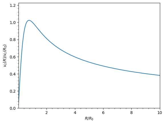
Let’s start by initializing a Miyamoto-Nagai disk potential and plotting its rotation curve. The normalize=1. option normalizes the potential so that the circular velocity equals 1 at R=1 (in galpy’s natural units).

from galpy.potential import MiyamotoNagaiPotential

mp = MiyamotoNagaiPotential(a=0.5, b=0.0375, normalize=1.0)
mp.plotRotcurve(Rrange=[0.01, 10.0], grid=1001);

Combining multiple potentials

A realistic galaxy model requires multiple components. We can combine potentials simply by adding them with +. Here we create a three-component model with a disk, a halo, and a bulge. Note that the normalize values sum to 1, so the composite circular velocity is 1 at R=1.

from galpy.potential import NFWPotential, HernquistPotential

mp = MiyamotoNagaiPotential(a=0.5, b=0.0375, normalize=0.6)
nfp = NFWPotential(a=4.5, normalize=0.35)
hp = HernquistPotential(a=0.6 / 8, normalize=0.05)
(hp + mp + nfp).plotRotcurve(Rrange=[0.01, 10.0], grid=1001, yrange=[0.0, 1.2]);

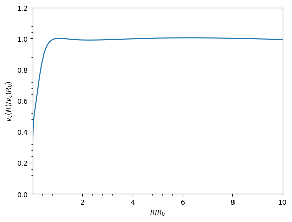
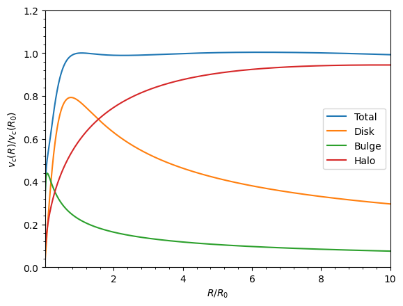
The resulting rotation curve is approximately flat, as observed in many spiral galaxies. We can overplot the individual component curves to see how each contributes:

(hp + mp + nfp).plotRotcurve(
    Rrange=[0.01, 10.0], grid=1001, yrange=[0.0, 1.2], label="Total"
)
mp.plotRotcurve(Rrange=[0.01, 10.0], grid=1001, overplot=True, label="Disk")
hp.plotRotcurve(Rrange=[0.01, 10.0], grid=1001, overplot=True, label="Bulge")
nfp.plotRotcurve(Rrange=[0.01, 10.0], grid=1001, overplot=True, label="Halo")
plt.legend();

MWPotential2014

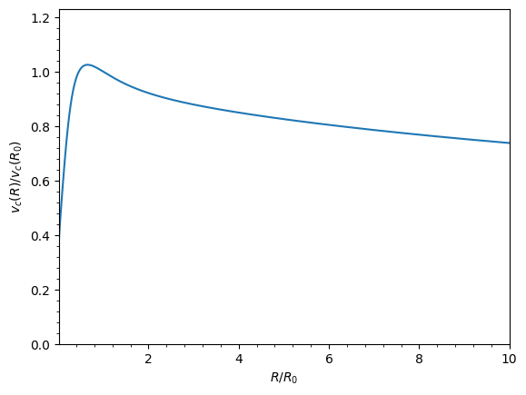
galpy includes MWPotential2014, a Milky-Way-like potential fit to various dynamical constraints (Bovy 2015). See the Introduction to Potentials for details.

from galpy.potential import MWPotential2014

MWPotential2014.plotRotcurve(Rrange=[0.01, 10.0], grid=1001);

2. Natural Units

Internally, galpy uses a natural unit system, where:

• Positions are scaled as $x = X / $ ro

• Velocities are scaled as $v = V / $ vo,

where the default values of ro and vo are 8 kpc and 220 km/s, respectively. These can be changed when initializing potentials, orbits, or other galpy objects or they can be changed in the configuration file. So when normalize=1. is set, the circular velocity is 1 at R=1, which corresponds to 220 km/s at 8 kpc for a Milky-Way-like galaxy.

The galpy.util.conversion module helps convert between natural and physical units. For example, the orbital period of a circular orbit at R=1 is \(2\pi\) in natural units. In physical units:

from galpy.util import conversion

print(
    "Orbital period at R=1:", 2.0 * numpy.pi * conversion.time_in_Gyr(220.0, 8.0), "Gyr"
)

Orbital period at R=1: 0.22340544439051707 Gyr

About 223 Myr, as expected for a solar-like orbit.

We can also convert forces and densities. For example, the vertical force at 1.1 kpc above the plane at the solar radius in MWPotential2014:

Fz = -MWPotential2014.zforce(1.0, 1.1 / 8.0)
print("Fz in pc/Myr^2:", Fz * conversion.force_in_pcMyr2(220.0, 8.0))
print("Fz in 2*pi*G*Msun/pc^2:", Fz * conversion.force_in_2piGmsolpc2(220.0, 8.0))

Fz in pc/Myr^2: 2.0259181889046634
Fz in 2*pi*G*Msun/pc^2: 71.67605643105574

The conversion module also has functions for densities (dens_in_msolpc3), masses (mass_in_msol), surface densities, and frequencies. See the API documentation for a full list.

3. Physical Units with astropy

Any input to a galpy Potential, Orbit, or other object can be specified in physical units using astropy Quantities. For example, we can set up a Miyamoto-Nagai potential with a mass of \(5 \times 10^{10}\,M_\odot\), a scale length of 3 kpc, and a scale height of 300 pc:

from astropy import units

mp_phys = MiyamotoNagaiPotential(
    amp=5e10 * units.Msun, a=3.0 * units.kpc, b=300.0 * units.pc
)

When a potential is set up with physical-unit inputs, outputs are returned in physical units by default. The circular velocity at 10 kpc:

print("v_circ at 10 kpc:", mp_phys.vcirc(10.0 * units.kpc), "km/s")

v_circ at 10 kpc: 135.70512798497137 km/s

If you have astropy-units = True in your galpy configuration file, the return value will be an astropy Quantity with units attached. Without that setting, the value is returned as a plain float in the default units (km/s for velocities, kpc for distances, etc.).

Warning

If you do not specify arguments as a Quantity, galpy assumes they are in natural units. For example, mp_phys.vcirc(10.) treats the input as 10 times the distance scale (80 kpc by default), not 10 kpc.

Default physical units

When outputs are returned in physical units, the following default units are used:

Quantity	Default unit
position	kpc
velocity	km/s
angular velocity	km/s/kpc
energy	(km/s)^2
angular momentum	km/s x kpc
actions	km/s x kpc
frequencies	1/Gyr
time	Gyr
period	Gyr
potential	(km/s)^2
force	km/s/Myr
density	Msun/pc^3
surface density	Msun/pc^2
mass	Msun
proper motion	mas/yr

Warning

When returned as a Quantity, frequencies get units of 1/Gyr, although in detail this means rad/Gyr (not cycles/Gyr).

Tip

When you specify all inputs as astropy Quantities with units and receive outputs as Quantities, the internal unit-conversion parameters ro and vo are irrelevant – you do not need to set them.

Toggling physical units on and off

You can toggle physical-unit output on or off for an object, or override it per call using the use_physical keyword. You can also pass quantity=True to any evaluation to get the result as an astropy Quantity.

mp_phys.turn_physical_off()
print("Natural units:", mp_phys.vcirc(1.0))
mp_phys.turn_physical_on()
print("Physical units:", mp_phys.vcirc(1.0), "km/s")
# Per-call overrides:
print(
    "Per-call override of use_physical:",
    mp_phys.vcirc(10.0 * units.kpc, use_physical=False),
)
print("Per-call override of quantity:", mp_phys.vcirc(10.0 * units.kpc, quantity=True))

Natural units: 0.6623918492376609
Physical units: 145.7262068322854 km/s
Per-call override of use_physical: 0.616841490840779
Per-call override of quantity: 135.70512798497137 km / s

4. First Orbit Integration

Let’s integrate an orbit in the Miyamoto-Nagai potential. We initialize an orbit with a five-dimensional initial condition [R, vR, vT, z, vz] (axisymmetric, so no azimuth):

from galpy.orbit import Orbit

mp = MiyamotoNagaiPotential(a=0.5, b=0.0375, amp=1.0, normalize=1.0)
o = Orbit([1.0, 0.1, 1.1, 0.0, 0.1])
ts = numpy.linspace(0, 100, 10000)
o.integrate(ts, mp)
o.plot();

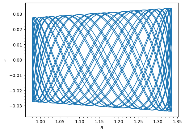
The orbit plot shows R vs. z. We can check energy conservation:

o.plotE(normed=True);

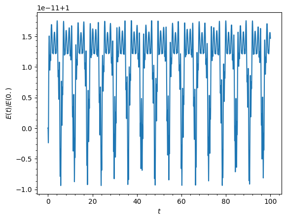
Energy is well conserved. See the Orbit Integration and Plotting tutorial for more on integrators and energy conservation.

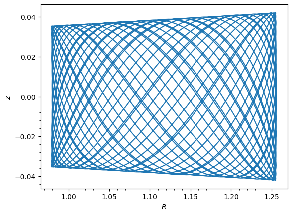
We can also integrate in the composite potential defined earlier:

mp = MiyamotoNagaiPotential(a=0.5, b=0.0375, normalize=0.6)
nfp = NFWPotential(a=4.5, normalize=0.35)
hp = HernquistPotential(a=0.6 / 8, normalize=0.05)
o = Orbit([1.0, 0.1, 1.1, 0.0, 0.1])
ts = numpy.linspace(0, 100, 10000)
o.integrate(ts, mp + hp + nfp)
o.plot();

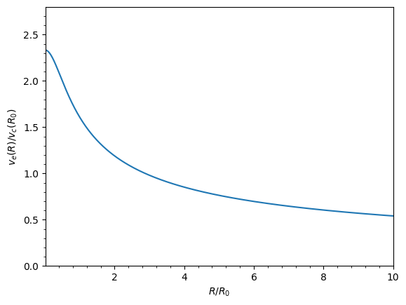
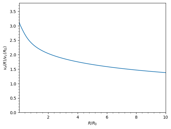
5. Escape Velocity Curves

Just like rotation curves, we can plot escape velocity curves for any potential or combination of potentials:

mp_single = MiyamotoNagaiPotential(a=0.5, b=0.0375, normalize=1.0)
mp_single.plotEscapecurve(Rrange=[0.01, 10.0], grid=1001);

We can do the same for the MWPotential2014 composite potential:

MWPotential2014.plotEscapecurve(Rrange=[0.01, 10.0], grid=1001);

The escape velocity at the solar radius in MWPotential2014:

v_esc = MWPotential2014.vesc(1.0)
print("Escape velocity at R=1 (natural units):", v_esc)
print("Escape velocity at solar radius:", v_esc * 220.0, "km/s")

Escape velocity at R=1 (natural units): 2.3316389848832784
Escape velocity at solar radius: 512.9605766743213 km/s

This is approximately 513 km/s, consistent with direct measurements of the Milky Way’s escape velocity (e.g., Smith et al. 2007; Piffl et al. 2014).

---

Next steps

Explore the rest of galpy’s documentation:

• Introduction to Potentials — evaluate potentials, forces, densities, and orbital frequencies

• Orbit Initialization — initialize orbits from various coordinate systems

• Milky Way-like Potentials — built-in models for the Milky Way

• Action-Angle Coordinates — compute orbital actions, frequencies, and angles