Welcome to galpy’s documentation
galpy is a Python package for galactic dynamics. It supports orbit integration in a variety of potentials, evaluating and sampling various distribution functions, and the calculation of action-angle coordinates for all static potentials. galpy is an astropy affiliated package and provides full support for astropy’s Quantity framework for variables with units.
galpy is developed on GitHub. If you are looking to report an issue, join the galpy slack community, or for information on how to contribute to the code, please head over to galpy’s GitHub page for more information.
Try galpy
Give galpy a try in the interactive IPython-like shell below!
Plot the rotation curve of the Milky Way
>>> from galpy.potential import (plotRotcurve,
        MWPotential2014 as mwp14)
>>> import matplotlib.pyplot as plt
>>> plotRotcurve(mwp14)
>>> plotRotcurve(mwp14[0],label='Bulge',overplot=True)
>>> plotRotcurve(mwp14[1],label='Disk',overplot=True)
>>> plotRotcurve(mwp14[2],label='Halo',overplot=True)
>>> plt.legend()
or integrate the orbit of MW satellites
>>> from galpy.orbit import Orbit
>>> from galpy.potential import MWPotential2014
>>> import numpy
>>> ts= numpy.linspace(0.,5.,2001)*u.Gyr
>>> o= Orbit.from_name('MW satellite galaxies')
>>> o.integrate(ts,MWPotential2014)
>>> o.plot(xrange=[0.,100.],yrange=[-100.,100.])
>>> o[o.name=='LMC'].plot(c='r',lw=5.,overplot=True)
or calculate the Sun's orbital actions, frequencies, and angles
>>> from galpy.orbit import Orbit
>>> from galpy.potential import (
        MWPotential2014 as mwp14)
>>> o= Orbit()
>>> print(o.jr(pot=mwp14),o.Lz(),o.jz(pot=mwp14))
>>> print(o.Or(pot=mwp14),o.Op(pot=mwp14),o.Oz(pot=mwp14))
>>> print(o.wr(pot=mwp14),o.wp(pot=mwp14),o.wz(pot=mwp14))
and much more... Start your journey below
>>> from galpy.potential import (plotRotcurve,
MWPotential2014 as mwp14)
>>> import matplotlib.pyplot as plt
>>> plotRotcurve(mwp14)
>>> plotRotcurve(mwp14[0],label='Bulge',overplot=True)
>>> plotRotcurve(mwp14[1],label='Disk',overplot=True)
>>> plotRotcurve(mwp14[2],label='Halo',overplot=True)
>>> plt.legend()>>> from galpy.orbit import Orbit
>>> from galpy.potential import MWPotential2014
>>> import numpy
>>> ts= numpy.linspace(0.,5.,2001)*u.Gyr
>>> o= Orbit.from_name('MW satellite galaxies')
>>> o.integrate(ts,MWPotential2014)
>>> o.plot(xrange=[0.,100.],yrange=[-100.,100.])
>>> o[o.name=='LMC'].plot(c='r',lw=5.,overplot=True)or calculate the Sun's orbital actions, frequencies, and angles
>>> from galpy.orbit import Orbit
>>> from galpy.potential import (
MWPotential2014 as mwp14)
>>> o= Orbit()
>>> print(o.jr(pot=mwp14),o.Lz(),o.jz(pot=mwp14))
>>> print(o.Or(pot=mwp14),o.Op(pot=mwp14),o.Oz(pot=mwp14))
>>> print(o.wr(pot=mwp14),o.wp(pot=mwp14),o.wz(pot=mwp14))and much more... Start your journey below
Quick-start guide
Install galpy on Linux, Mac, or Windows via pip or conda, including optional C extensions and configuration. Development installation from source and development setup.
High-level release notes for all galpy versions.

Set up basic potentials, plot rotation curves, understand galpy’s natural and physical unit systems, and integrate a simple orbit.
Potentials

Evaluate potentials, forces, and densities. Combine potentials, plot rotation curves and potential contours, compute orbital frequencies and Lindblad resonances.

Use built-in Milky Way potentials: MWPotential2014, McMillan17, Irrgang13, Cautun20, DehnenBinney98. Add a central black hole or dynamical friction.

Modify potentials with time-dependent amplitudes, solid-body rotation, tilting, and offsetting using wrapper classes.

Represent arbitrary density distributions using basis-function (SCF) or multipole expansions, including time-dependent and disky potentials.

Use velocity-dependent forces like Chandrasekhar dynamical friction and non-inertial frame forces for orbit integration. Includes the Schwarzschild precession of S2 around Sgr A*.

Use frozen N-body simulation potentials in galpy with pynbody for orbits, action-angle coordinates, and analysis.
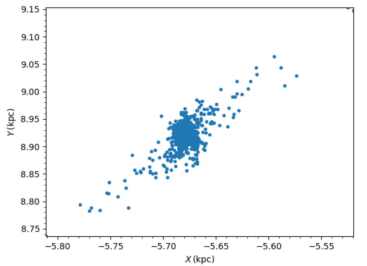
Export galpy potentials to NEMO, AMUSE, AGAMA, and gala for use in other simulation frameworks.
Orbits

Initialize orbits in cylindrical coordinates, with physical units, from observed coordinates (RA/Dec, Galactic), or from astropy SkyCoord objects.

Work with multiple orbits at once: array and SkyCoord initialization, slicing, reshaping, and parallel integration.

Initialize orbits from object names using built-in catalogs or SIMBAD. Load collections of MW globular clusters, satellite galaxies, or the solar system.

Integrate orbits, display various projections, access orbital quantities, check energy conservation, use non-inertial frames, and compute surfaces of section.

Quickly compute eccentricity, peri/apocenter, and zmax using the Staeckel approximation without orbit integration. Also compute actions!
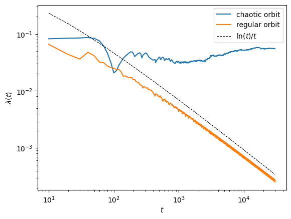
Integrate phase-space deviations in 2D and 3D with the variational equations, verify Liouville’s theorem, and compute Lyapunov exponents to detect chaos.

Detailed examples: thick-disk eccentricity distribution, LMC orbit with dynamical friction, and barycentric acceleration from the LMC.
Action-Angle Coordinates

Overview of action-angle variables, using the Orbit interface, calculating actions for isochrone and spherical potentials, and exact inverse transforms in the isochrone case.

The most accurate general method for computing actions in axisymmetric potentials, with grid-based interpolation for speed. Includes a Gaia example showing Lindblad resonances.

Fast action calculation by separating radial and vertical motions, best for thin-disk orbits.

General action-angle calculation by integrating the orbit and using a best-fit isochrone potential.

One-dimensional action-angle coordinates for harmonic oscillators and vertical oscillations, and their inverse transformations.

Compute phase-space coordinates from given actions and angles using the Torus Mapper.
Distribution Functions

Dehnen, Shu, and Schwarzschild distribution functions for razor-thin disks: moments, asymmetric drift, Oort constants, sampling, and non-axisymmetric evolution.

Quasi-isothermal distribution function for 3D disk populations using action-angle variables: moments, velocity ellipsoid tilt, and velocity sampling.

Isotropic and anisotropic distribution functions for spherical systems: Hernquist, NFW, King, Plummer, Power-law, and general models. Includes N-body initial conditions for a truncated NFW halo and a two-component dwarf galaxy (stars embedded in dark matter).
Tidal Streams

Model tidal streams in action-angle coordinates: predict stream tracks, compute densities, sample mock data, and evaluate the full phase-space PDF. And model gaps.

Generate tidal streams using particle-spray techniques with chen24spraydf and fardal15spraydf.
Extending galpy

Define custom potential classes and dissipative forces in Python by implementing force and potential evaluation methods, with full support for orbit integration and physical units.
Add C implementations of potentials for fast orbit integration and action-angle calculations.
Library reference
- Orbit (
galpy.orbit) - Potential (
galpy.potential) - actionAngle (
galpy.actionAngle) - DF (
galpy.df)- Jeans modeling tools (
galpy.df.jeans) - General instance routines for all df classes
- Spherical distribution functions
- Two-dimensional, axisymmetric disk distribution functions
- Two-dimensional, non-axisymmetric disk distribution functions
- Three-dimensional disk distribution functions
- The distribution function of a tidal stream in action-angle coordinates
- The distribution function of a gap in a tidal stream
- The distribution function of a tidal stream using a particle-spray technique
- Jeans modeling tools (
- Utilities (
galpy.util)
Acknowledging galpy
If you use galpy in a publication, please cite the following paper
galpy: A Python Library for Galactic Dynamics, Jo Bovy (2015), Astrophys. J. Supp., 216, 29 (arXiv/1412.3451).
and link to http://github.com/jobovy/galpy. Some of the code’s
functionality is introduced in separate papers:
galpy.actionAngle.EccZmaxRperiRapandgalpy.orbit.Orbitmethods withanalytic=True: Fast method for computing orbital parameters: please cite Mackereth & Bovy (2018).galpy.actionAngle.actionAngleAdiabatic: please cite Binney (2010).galpy.actionAngle.actionAngleStaeckel: please cite Bovy & Rix (2013) and Binney (2012).galpy.actionAngle.actionAngleIsochroneApprox: please cite Bovy (2014).galpy.df.streamdf: please cite Bovy (2014).galpy.df.streamgapdf: please cite Sanders, Bovy, & Erkal (2016).galpy.df.chen24spraydf: please cite Chen et al. (2024) for the method and thegalpyimplementationgalpy.df.fardal15spraydf: please cite Fardal et al. (2015) for the method and Qian et al. (2022) for thegalpyimplementationgalpy.potential.ttensorandgalpy.potential.rtide: please cite Webb et al. (2019a).galpy.potential.to_amuse: please cite Webb et al. (2019b).
Please also send me a reference to the paper or send a pull request including your paper in the list of galpy papers on this page (this page is at doc/source/index.rst). Thanks!
Papers using galpy
galpy has been used in more than 200 scientific publications in the astrophysical literature. Covering topics as diverse as the properties of planetary systems around distant stars, the kinematics of pulsars and stars ejected from the Milky Way by supernova explosions, binary evolution in stellar clusters, chemo-dynamical modeling of stellar populations in the Milky Way, and the dynamics of satellites around external galaxies, galpy is widely used throughout astrophysics.
Check out the gallery below for examples: